Paid course

Power Converter Efficiency

Name: Power Converter Efficiency
Price: 19 EUR
Availability: InStock

Learn how to calculate converter losses and combine them into an efficiency map. A synchronous buck converter is used as the worked example. Chapters 1 and 2 are free.

Welcome

Efficiency tells you how much of the power going into a converter actually reaches the output: \[ \eta = \frac{P_{out}}{P_{in}}. \] So if a converter is 97 % efficient, the remaining 3 % has gone somewhere else. Most of it becomes heat. That may sound like a small amount, but around a kilowatt, even a few percent means tens of watts of heat. That is enough to affect how hot the components run and how long they last.

This course is about finding that missing power. We use one synchronous buck converter as the running example and build its loss budget one part at a time. Once that way of thinking makes sense, you can use the same method for other power converters as well.

The buck converter used in this course

Our buck converter steps three different input voltages down to 50 V. We look at how its losses change as output power rises from 100 W to 1250 W. For each input voltage, only output power changes; the other model inputs stay fixed. The buck WebSimulator supplies currents at each power point; the efficiency calculator then evaluates the losses from those results. Unless a plot says otherwise, we use 25 °C as the ambient-temperature reference, without modelling self-heating.

Open the buck operating-point cases. The test selector contains all 18 input-voltage/load combinations. Load values are requested operating points; the simulator’s achieved voltage and current can differ slightly because switching is resolved in discrete time steps.

Figure 1Course buck converter current paths: input path, switching leg, inductor, output path, and capacitor-current paths.

These are the numbers behind the plots and examples:

Quantity	Value or relationship
Input voltage $V_{in}$	80 / 100 / 120 V
Output voltage $V_{out}$	50 V
Output power $P_{out}$	100 W to 1250 W
Output current $I_{out}$	$I_{out}=P_{out}/V_{out}$, 2 A to 25 A
Ideal buck duty $D$	$D\approx V_{out}/V_{in}$, 0.417 to 0.625
Switching frequency $f_{sw}$	50 kHz
Inductor $L_1$	38 turns on Magnetics Kool Mµ 0077439A7; inductance varies with current
Switches $Q_1$, $Q_2$	onsemi NTH4L012N065M3S SiC MOSFETs, synchronous pair
Cooling	One fan

The table is a reference for the examples throughout the course. Alongside the main power components, our budget includes connectors, the fuse, the current shunt, control electronics, and the fan. To keep this example simple, we leave out PCB-track and capacitor losses.

Course organization

We start with an overview of the losses, then work through the components and calculations behind them.

Chapter 1: The loss families and why the efficiency curve has its shape.
Chapter 2: The components that carry current and produce loss.
Chapter 3: Why conduction loss grows quickly with current and temperature.
Chapter 4: What happens inside the inductor core.
Chapter 5: What is lost each time the switches change state.
Chapter 6: The power used by the auxiliary electronics and cooling.
Chapter 7: How the losses are measured and calculated.
Chapter 8: How to rank losses by component, compare switching frequencies, and use the budget to improve the design.

Chapter 01

The five loss families

Every watt that does not reach the output ends up somewhere. In this course, we sort that missing power into five groups: conduction, core, switching, auxiliary, and cooling loss.

Before calculating each part, it helps to see what changes with load. In our model, some losses stay almost constant while others grow with current. Their relative sizes explain why efficiency changes as output power rises.

Conduction loss

Whenever current flows through resistance, some power becomes heat: \[ P_{cond}=I^2R. \] The important part is the square on the current. For the same resistance, doubling the current gives four times the loss. At low output power, conduction loss is small, but it climbs quickly as the current rises. Near full load, it often becomes the largest loss in the converter.

The resistance is spread across the whole current path: the switches, inductor winding, fuse, connectors, PCB copper, and current shunt all add a little more.

Figure 2Conduction loss in the L1 winding grows with current squared.Open in loss calculator ↗

Core loss

The magnetic field inside the inductor core rises and falls during every switching cycle. Each cycle loses a little energy as heat in the core. The voltage across the winding and the switching frequency affect the size of the magnetic swing: \[ \Delta B\propto\frac{V_L}{f_{sw}}. \] $\Delta B$ is the size of that magnetic swing. For the same inductor and duty cycle, a larger voltage across the winding makes the swing larger. A higher switching frequency leaves less time for it to change in each cycle, making the swing smaller.

Within each load sweep here, all model inputs except output power stay fixed. The magnetic swing then stays almost unchanged, so the model gives nearly constant core loss as output power rises. That does not make core loss a fixed property of the inductor: changing the input or output voltage changes the voltage across its winding and can change the loss.

Figure 3Core loss versus output power at different input voltages. Other model inputs stay fixed.Open in loss calculator ↗

Switching frequency changes two things at once: how often the core goes through a cycle, and how large the magnetic swing is. In this example, the smaller swing outweighs the extra cycles, so increasing frequency reduces the core-loss term. Switching loss rises with frequency, though, so this does not mean the converter’s total loss falls.

Figure 4Core loss versus output power at different switching frequencies. Other model inputs stay fixed.Open in loss calculator ↗

Switching loss

A switch cannot change state instantly. For a short moment during each transition, it has voltage across it while current is flowing through it. That overlap becomes heat: \[ P_{sw}=f_{sw}(E_{on}+E_{off}). \] Each transition costs a small amount of energy. Switching more often repeats that cost more times per second. Higher current and higher switched voltage usually make each transition more expensive too. Chapter 5 works through the device data and the detailed calculation.

Figure 5The shaded overlap during turn-on and turn-off is the energy lost in each switching transition.

Auxiliary power

The controller, sensors, and their power supplies need power just to keep the converter running. That auxiliary power changes little with output power in this model. At light load, even a small fixed loss is a large share of the power being delivered. At high load, the same loss becomes much less important.

Figure 6The auxiliary supply powers the controller and gate driver. The controller tells the driver when to switch the power MOSFET.

Cooling loss

The fan helps remove the heat produced inside the converter. As output power rises, this converter produces more heat. Increasing fan power is one way to provide the extra cooling.

There are several ways to control a fan. For this course, we use one simple assumption: fan power increases linearly with output power. That is a model choice, not a rule that every real fan controller must follow. The fan still uses input power, so its consumption belongs in the complete loss budget.

Figure 7Fan power rises with output power under the course’s linear control assumption.Open in loss calculator ↗

Total loss and efficiency

\[ \begin{aligned} P_{loss}={}&P_{cond}+P_{core}+P_{sw}\\ &+P_{aux}+P_{cool}. \end{aligned} \] \[ \eta=\frac{P_{out}}{P_{out}+P_{loss}}. \] The plot below puts all five families together. Its loss axis is logarithmic so the small losses remain visible beside the large ones.

Figure 8The five loss families across output power. The logarithmic axis keeps the smaller losses visible.Open in loss calculator ↗

These numbers are for our buck converter. Different components and circuits can change both the losses and which ones matter most. For example, a cheaper inductor might use a core material with higher loss or a winding with more resistance. It is those differences in construction that affect the loss.

This explains the shape of the efficiency curve. In this output-power sweep, auxiliary and core loss are approximately fixed. As those fixed losses become a smaller fraction of the output power, efficiency improves. Cooling is not fixed: this course model makes fan power rise linearly with output power, so its fraction stays roughly constant. At high power, conduction loss catches up because it grows with current squared, and the efficiency curve bends down again.

Figure 9Efficiency across output power for the course’s three input-voltage cases.Open in loss calculator ↗

Temperature matters too. As copper warms up, its resistance rises. At the same current, that means more conduction loss. The plot shows $R/R_{20}$, the resistance divided by its value at 20 °C. A value of 1 means the resistance at 20 °C; 1.2 means it is 20 % higher.

$Copper resistance relative to its value at 20 °C: $R/R_{20}=1$ at the reference temperature.$

Figure 10Copper resistance relative to its value at 20 °C: $R/R_{20}=1$ at the reference temperature.Open in loss calculator ↗

The MOSFETs used here also become more resistive as they warm up, though they follow a different curve from copper. Switching and core losses have their own temperature behaviour, which depends on the device and magnetic material. We come back to those details in the later chapters.

Key idea

In this converter, nearly constant losses matter most at light load. At high load, conduction loss takes over because it grows with current squared. That shift gives the efficiency curve its shape.

Loss budget at 100 W and 1250 W

The two ends of the course sweep show how the balance changes between low and high output power. Only output power changes. All other model inputs are held constant.

Figure 11The loss budget at two loads. The percentages are the share of each panel’s total.Open in loss calculator ↗

Family	100 W output	1250 W output
Conduction	0.12 W	16.92 W
Switching	1.00 W	2.87 W
Core	0.45 W	0.45 W
Auxiliary	0.86 W	0.86 W
Cooling	0.20 W	2.40 W
Total loss	2.62 W	23.49 W
Efficiency	97.44 %	98.16 %

At 100 W, switching and auxiliary power are the largest contributions in this example. At 1250 W, conduction is clearly the largest family. Cooling grows with output power; it is not part of the fixed-loss contribution.

In a sentence

The shape of the efficiency curve comes from losses that behave differently. Knowing which ones are nearly fixed, which change with voltage or frequency, and which grow with current squared gives us a starting point for the component calculations.

Chapter 02

Representative components and current paths

We will keep the circuit in three parts: the input side, the half bridge, and the output filter and connection. Each section below shows that part of the schematic and explains the components inside it.

Figure 12The course schematic, divided into the input, switching stage, and inductor/output path.

Part	Component and model	Relevant values
X1, X2	PCB connector: Amphenol PwrBlade+ 10106124-4004001LF	1.4 mΩ per outgoing/return pair; each path has its own pair
F1	Fuse: Littelfuse 0505025.MXP	4.8 mΩ nominal cold resistance
C1	Film capacitor bank: TDK B32678T3306K000	2 × 30 µF = 60 µF; ESR loss omitted
Q1, Q2	SiC MOSFET: onsemi NTH4L012N065M3S	12 mΩ typical each at 25 °C, 18 V gate drive; manufacturer $E_{on}$ and $E_{off}$ curves
L1	Custom winding: 38 turns on Magnetics 0077439A7	10.8 mΩ at 20 °C; about 195 µH near zero current, 83 µH at 25 A
C2	Electrolytic capacitor: Nichicon UCY2D471MHD	470 µF; ESR loss omitted
R2	Current shunt: Bourns CSS2H-2512R-1L00F	1.0 mΩ

These are the same component values used later and in the calculator. L1’s winding resistance and inductance are calculated for our custom winding, not specifications for a ready-made inductor. The sections below explain each component and the conditions behind its value.

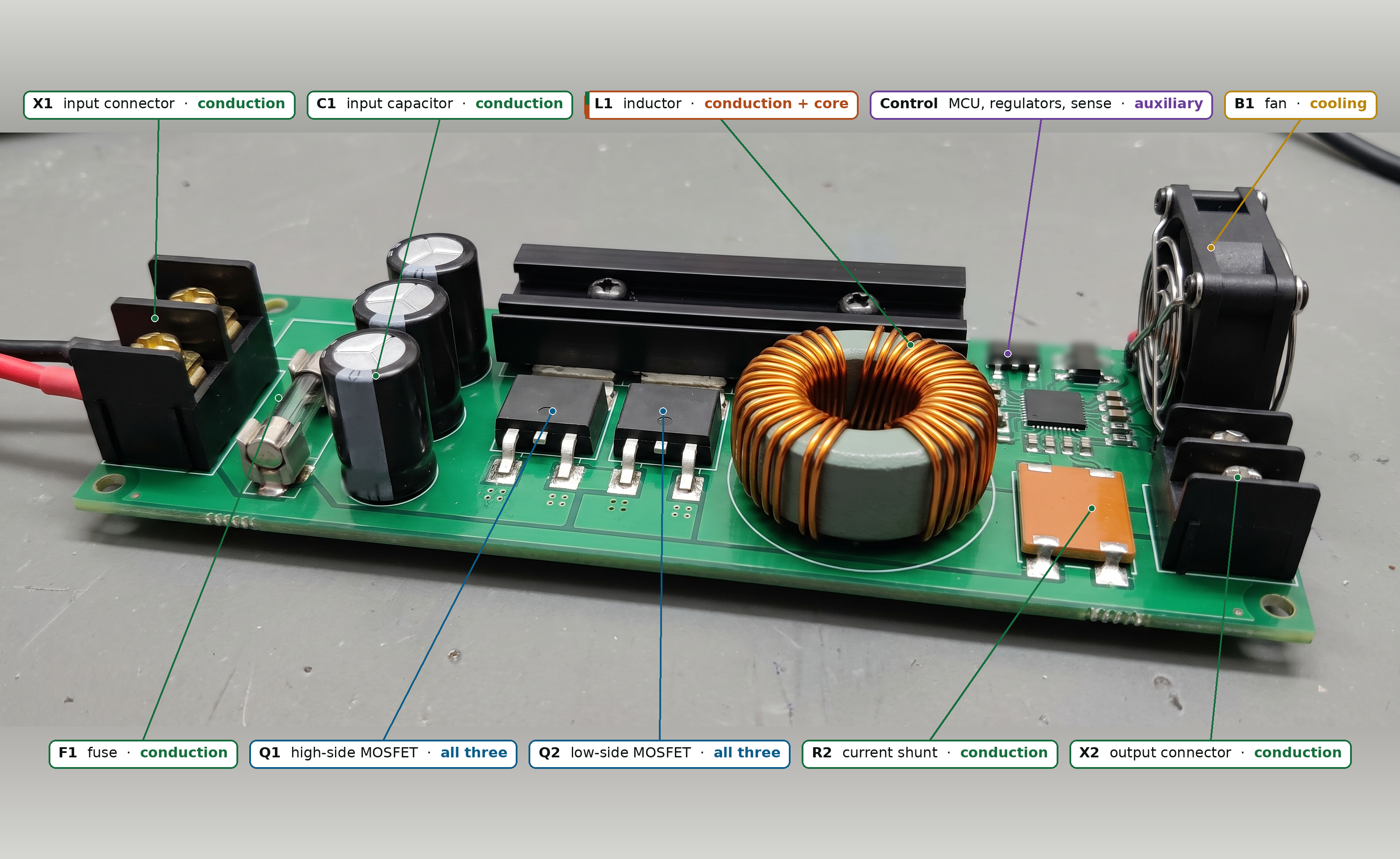
AI-generated illustration. An example of a complete buck-converter board. The components shown are only for illustration, not the specific parts used in the calculations later in this course.

Figure 13AI-generated illustration. An example of a complete buck-converter board. The components shown are only for illustration, not the specific parts used in the calculations later in this course.

The links below take you to the component details. We’ll use the resistances shown here in the loss calculations, rather than a separate set of course values. This is still an example design, not a complete build specification.

The input side

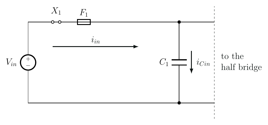
Figure 14The input section: connector X1, fuse F1 and capacitor C1. The capacitor has its own ripple-current path.

X1: the input connector

The connector lets us connect the board to the power supply. Current passes through metal contacts, which have a small resistance and produce heat. Both the supply contact and the return contact count.

The Amphenol PwrBlade+ is a PCB-mounted power connector. Its terminals connect directly to the board, and a mating connector plugs into it. One example is the 10106124-4004001LF right-angle header. The large contacts carry power; the smaller ones carry signals.

This version has four power contacts, so one connector housing can carry both input and output: one pair for the supply and return, and a separate pair for the load and return. The contact ratings must suit both paths. We keep those two connections separate in the schematic as X1 and X2.

Manufacturer photograph: Amphenol. PwrBlade+ PCB connectors, showing the power contacts and smaller signal contacts. Image from the linked family datasheet.

Figure 15Manufacturer photograph: Amphenol. PwrBlade+ PCB connectors, showing the power contacts and smaller signal contacts. Image from the linked family datasheet.

For our calculations, we use the same resistance for the input and output:

\[R_{X1} = R_{X2} = 1.4\,\mathrm{m}\Omega.\]

The datasheet gives a maximum of 0.7 mΩ per power contact. Two contacts make 1.4 mΩ for each path, including outgoing and return, not input and output combined. We use that limit as the starting resistance in the calculations.

F1: the fuse

A fuse interrupts the current if an overload heats its element enough to melt it. That element also has resistance during normal operation, so a fuse contributes conduction loss even when nothing is wrong.

The Littelfuse 0505025.MXP is our 25 A ceramic-cartridge example. It leaves more continuous-current margin than the earlier 20 A choice at the lowest input voltage.

AI-generated illustration. A ceramic cartridge fuse. The white body contains the fuse element; the metal end caps connect it to its holder.

Figure 16AI-generated illustration. A ceramic cartridge fuse. The white body contains the fuse element; the metal end caps connect it to its holder.

Its nominal cold resistance is the value we’ll use:

\[R_{F1} = 4.8\,\mathrm{m}\Omega.\]

C1: the input capacitor

A capacitor stores electrical energy and can take in or supply current to help keep a voltage steady. C1 sits across the input rails and carries ripple current. That is not the same current as the average current coming from the supply.

Here C1 represents two TDK B32678T3306K000 film capacitors in parallel: 30 µF each, or 60 µF total. We chose a film-capacitor bank because this input position carries substantial ripple current.

Manufacturer illustration: TDK/EPCOS. A boxed film capacitor from the B3267 family. C1 uses two 30 µF capacitors in parallel; this shows the package type, not the complete bank.

Figure 17Manufacturer illustration: TDK/EPCOS. A boxed film capacitor from the B3267 family. C1 uses two 30 µF capacitors in parallel; this shows the package type, not the complete bank.

Ripple current heats the capacitor’s internal resistance, called ESR. We leave capacitor losses out to simplify this example. They are not zero, and a real design still needs a ripple-current and heating check.

The half bridge

Figure 18The half bridge, containing Q1 and Q2. Its output connects to L1 in the next section.

Q1 and Q2: the MOSFETs

A MOSFET is an electronic switch. A control signal at its gate tells it whether to conduct current. Q1 and Q2 are the two switches in this part of the schematic; we use the same component type for both.

Even when a MOSFET is on, it has resistance. It also loses energy while switching, and charging its gate takes energy. Those are the three things we need to keep track of.

Our example uses the onsemi NTH4L012N065M3S. Its 650 V rating is much higher than this 120 V teaching converter needs, so it is not presented as a cost-optimised switch selection. We use it because it comfortably covers the current and voltage range and, importantly for this course, the manufacturer publishes the resistance, gate-charge, and current-dependent switching-energy curves needed for one consistent loss model.

AI-generated illustration. A surface-mount power MOSFET in a D²PAK-style package. The metal terminals connect the semiconductor to the board.

Figure 19AI-generated illustration. A surface-mount power MOSFET in a D²PAK-style package. The metal terminals connect the semiconductor to the board.

For both Q1 and Q2, we’ll use the typical on-resistance:

\[R_{\mathrm{DS(on)}} = 12\,\mathrm{m}\Omega.\]

This is the typical datasheet value at 25 °C with 18 V gate drive, measured at 40 A. Later, we’ll account for how resistance changes with temperature.

Gate-drive energy belongs to Q1 and Q2 physically, but this course classifies the power drawn from their gate-drive supply as auxiliary power. Chapter 6 calculates it there, so do not add it a second time under switching loss.

The output filter and connection

Figure 20The output section: L1 and C2 form the filter; R2 measures current and X2 connects to the load.

L1: the inductor

An inductor is a coil of wire, usually wound around a magnetic core. It stores energy in a magnetic field and helps smooth current.

The wire and core lose power for different reasons: resistance heats the winding, while the changing magnetic field heats the core. We keep those as separate loss terms.

Figure 21AI-generated illustration. A toroidal inductor: insulated copper wire wound around a ring-shaped core.

Our inductor has a custom 38-turn winding on a Magnetics 0077439A7 Kool Mµ core. That part number identifies the core, not a ready-wound inductor. For the winding in our example, we use this resistance at 20 °C:

\[R_{L1} = 10.8\,\mathrm{m}\Omega.\]

This is calculated for about 3 m of winding wire, including leads, with 4.8 mm² total copper area. It is not a resistance specified for the bare core or a measurement of a built inductor. The same value is used in the calculator. Later, we’ll account for the core’s changing inductance and calculate its magnetic loss separately.

The inductance is about 195 µH near zero current and 83 µH at 25 A, using the manufacturer’s typical DC-bias fit. It falls as current rises: this core does not keep the same inductance at every load.

C2: the output capacitor

C2 is another capacitor, now helping smooth the output voltage. Together, L1 and C2 form the output filter. Here we use a 470 µF Nichicon UCY2D471MHD aluminium electrolytic capacitor. Its ripple-current requirement is different from C1’s. We leave its loss out of the simplified budget too.

AI-generated illustration. A radial aluminium electrolytic capacitor, representative of the package used for C2. C1 uses film capacitors in a different package.

Figure 22AI-generated illustration. A radial aluminium electrolytic capacitor, representative of the package used for C2. C1 uses film capacitors in a different package.

R2: the current shunt

A shunt is a small resistor used to measure current. Current through it produces a small voltage that the measurement circuit can read. Lower resistance means less heat, but also a smaller signal to measure.

The Bourns CSS2H-2512R-1L00F is the shunt used in this example:

\[R_{R2} = 1.0\,\mathrm{m}\Omega.\]

Manufacturer photograph: Bourns. The CSS2H-2512 surface-mount current shunt. Its two metal terminals connect the low-resistance element to the PCB.

Figure 23Manufacturer photograph: Bourns. The CSS2H-2512 surface-mount current shunt. Its two metal terminals connect the low-resistance element to the PCB.

X2: the output connector

X2 connects the board to the load. We use the same contact-pair resistance as X1, as shown above. The two paths carry different currents, so they can produce different amounts of heat even if they share one connector housing.

In a sentence

Keep the three circuit sections in mind: input, half bridge, and output. Within each one, identify the components and where they lose power. That is the starting point for the calculations in the next chapters.

Continue with Chapters 3 to 8

The Welcome section and Chapters 1 and 2 are free. Purchase the course to continue with the detailed loss calculations and complete workflow.

Quantity	Value or relationship
Input voltage \(V_{in}\)	80 / 100 / 120 V
Output voltage \(V_{out}\)	50 V
Output power \(P_{out}\)	100 W to 1250 W
Output current \(I_{out}\)	\(I_{out}=P_{out}/V_{out}\), 2 A to 25 A
Ideal buck duty \(D\)	\(D\approx V_{out}/V_{in}\), 0.417 to 0.625
Switching frequency \(f_{sw}\)	50 kHz
Inductor \(L_1\)	38 turns on Magnetics Kool Mµ 0077439A7; inductance varies with current
Switches \(Q_1\), \(Q_2\)	onsemi NTH4L012N065M3S SiC MOSFETs, synchronous pair
Cooling	One fan