Weak grids, SCR, and why anyone pays for this
The usual story, and why this book is not going to lean on it
The usual pitch for grid-forming control goes: the grid is filling up with inverters replacing synchronous generators, the remaining grid is getting electrically “weaker” as a result, and grid-following inverters fall over on a weak grid because their PLL fights the grid impedance. That story is true. It is also, as this chapter will show honestly, not the reason this book’s own 5 kVA running example needs grid-forming control: at that scale, the grid it normally sees is very strong. Working through why that story is true at transmission scale, and why it does not carry down to a domestic battery inverter, is the fastest way to actually understand short-circuit ratio rather than just quote the slogan.
Short-circuit ratio, defined properly
Short-circuit ratio (SCR) compares the strength of the grid at a connection point with the size of the thing connecting to it: \[ SCR = \frac{S_{sc}}{S_n} \] where \(S_{sc}\) is the grid’s short-circuit apparent power at that point: how much fault current the grid could deliver there, and \(S_n\) is the rated power of the inverter. A national-laboratory survey of grid-strength metrics puts it plainly:
“Grid strength measures the ability of a power grid to sustain a fault on a given bus and thus recover from such events. Grid strength is measured in terms of the available short-circuit current or short-circuit power (MVA) at a given bus.”6
A large SCR means the grid at that point is stiff: a huge amount of short-circuit current is available relative to the unit’s own rating, so the unit’s own behaviour barely moves the local voltage. A small SCR means the opposite: the unit is a significant fraction of everything the grid can deliver at that point, and its own current materially moves its own terminal voltage.
A number that circulates constantly is “SCR above 3 is a strong grid.” The same NREL survey explicitly refuses to endorse it as a hard line:
“In general, there is no unique, clear threshold for SCR to distinguish a weak grid condition from a strong grid condition. A general rule of thumb is to classify a grid to be weak if \(SCR < 3\) and strong if \(SCR > 5\). Note that an SCR < 3 does not necessarily mean system will be unstable… Still, thanks to its simplicity, SCR can be used as a screening tool.”7
So: weak below 3, strong above 5, and a grey band in between, not a single line at 3. The same source adds the honest limitation of the metric itself: SCR is computed at one frequency (50 or 60 Hz) and says nothing about how the grid impedance behaves at other frequencies, so a unit can be unstable at an SCR the rule of thumb calls comfortable if the impedance shape elsewhere is wrong for its controller.
The sharpest published number for where grid-following genuinely stops working, and where grid-forming is expected to keep working, comes from a test standard rather than a rule of thumb. AEMO’s voluntary specification for grid-forming inverters sets its test floor at \(SCR = 1.25\), explaining the choice directly:
“An SCR of 1.25 was selected as the lower limit as it is below the SCR stability threshold of typical GFL devices but is above power transfer limits.”8
and requires that a grid-forming unit stay stable all the way down to that number, excusing it only below \(SCR = 1\), where a different limit (covered next) takes over regardless of controller.
The static half: why SCR = 1 is a hard wall
Take the same power-angle relation from Chapter 1, \(P \approx (EV/X)\sin\delta\), and use the definition \(SCR = V^2/(X\,P_n)\) to eliminate \(X\). Writing power in per unit of the plant’s own rating with \(E \approx V\): \[ \boxed{\ \frac{P}{P_n} = SCR \cdot \sin\delta\ } \]
This one line is worth sitting with, because it says something exact and memorable: at rated output, \(\sin\delta = 1/SCR\).
| SCR | \(\delta\) at rated output | \(dP/d\delta\) (pu per rad) |
|---|---|---|
| 5 | \(11.5^\circ\) | 4.90 |
| 3 | \(19.5^\circ\) | 2.83 |
| 2 | \(30.0^\circ\) | 1.73 |
| 1.5 | \(41.8^\circ\) | 1.12 |
| 1.25 | \(53.1^\circ\) | 0.75 |
| 1.0 | \(90.0^\circ\) | 0.00 |
\(SCR = 1\) is, literally, the nose of the power-angle curve at rated output: the point where the curve stops rising at all, so there is no angle that delivers more power, no matter what the controller does. This is exactly why AEMO picked 1.25 as the floor (“above power transfer limits”) and excuses tripping below 1.0: below that point you are not fighting a controller problem any more, you are fighting arithmetic.

Reactive power behaves the same way from a different door: a reactive injection \(\Delta Q\) moves the local voltage by \(\Delta V \approx (\Delta Q/P_n)/SCR\) per unit: at \(SCR = 2\), a 0.1 pu reactive step moves the terminal voltage by 5%. Weak grids are voltage-soft in exactly the sense that makes that intuitive.
The dynamic half: why a PLL fights a weak grid
The static picture above is exact and needs no small-signal machinery, but it is not the whole story: a grid-following inverter can go unstable even where the static power-transfer limit is nowhere near being reached, because its own current moves the very angle its PLL is trying to measure.
Express the injected current in the PLL’s own frame as \(i = i_d + j i_q\). The terminal voltage seen at the point of common coupling is \(v_{pcc} = v_g + jX_g\,i\), and the quadrature term \(jX_g i_d\) rotates the PCC voltage angle: \[ \Delta\theta_{pcc} \approx \frac{X_g\,i_d}{V} \approx \frac{P_{pu}}{SCR}. \]
The PLL locks to \(v_{pcc}\), not to \(v_g\): it has no other choice, that is the only voltage it can measure. So the PLL is chasing an angle that its own inverter’s current is moving. That is a feedback loop with gain \(\approx P_{pu}/SCR\), which reaches unity exactly at \(SCR \approx P_{pu}\): the same SCR \(\approx 1\) boundary, arriving this time from the dynamics rather than from statics. Below that, the loop is positive feedback and no amount of PLL retuning saves it; above it, whether the loop is actually stable comes down to phase margin, set by the PLL’s own bandwidth, which is exactly why “slow the PLL down on a weak grid” is standard practice, and exactly why it trades away the very speed a fast PLL was built to provide.9
None of the dq-impedance machinery used to formalise this (impedance matrices, mirror-frequency coupling, a Nyquist test on the loop) presumes anything beyond a three-phase balanced Park transform, so it does not transfer to a single-phase PLL unchanged: a single-phase synchronising loop is built from an orthogonal-signal generator (Chapter 3 introduces this) and has to be re-analysed in the stationary frame. The mechanism above (a converter’s own current rotating the voltage it is trying to measure) transfers exactly; the specific dq analysis tools do not.
The duality, stated as a trade rather than a verdict
Chapter 1 already flagged the shape of this. A rigorous treatment of the two control philosophies as duals of each other states it precisely:
“A grid-forming inverter (voltage-forming, current-following) is vulnerable to a strong grid and cannot operate with short-circuit… As a dual, a grid-following inverter (current-forming, voltage-following) is vulnerable to a weak grid and cannot operate with open-circuit.”10
| Grid-forming | Grid-following | |
|---|---|---|
| Stable extreme | Open circuit (\(Z_g\to\infty\)), or an ideal current source at its terminals | Short circuit (\(Y_g\to\infty\)), or an ideal voltage source at its terminals |
| Unstable extreme | Short circuit (\(Z_g = 0\)), or an ideal voltage source at its terminals | Open circuit (\(Y_g = 0\)), or an ideal current source at its terminals |
| Fails as the grid gets… | strong | weak |
| Fights its own… | droop/synchronising gain | PLL bandwidth |
| Wants its inner loop… | voltage-bandwidth kept high | current-bandwidth kept high |
The corollary is worth saying out loud, because marketing material tends to erase it: “grid-forming is just better” is false as a general statement. A grid-forming inverter with a large droop gain hard-wired directly across a very stiff bus is unstable for exactly the same underlying reason a grid-following inverter is unstable on a very weak one: each control philosophy wants more series impedance between itself and the thing it is fighting to stay decoupled from; grid-following wants less.
The honest motivation, at this book’s own scale
Here is the number that changes everything about how this chapter should be read for a 5 kVA unit. A typical domestic low-voltage connection has a loop impedance somewhere around \(0.4\)-\(0.8\ \Omega\) at 230 V.
This book’s nominal grid-side inductance is \(L_g = 1.5\ \mathrm{mH}\), giving \(X_g = \omega L_g = 2\pi\times 50\times 0.0015 = 0.471\ \Omega\) (this is a simplification: real LV feeders are resistance-dominated, and Chapter 10 corrects for that; treating the loop as purely reactive here keeps the SCR calculation clean). The short-circuit apparent power at the PCC is \[ S_{sc} = \frac{V_n^2}{X_g} = \frac{230^2}{0.471} \approx 112\ \mathrm{kVA} \] \[ SCR = \frac{S_{sc}}{S_n} = \frac{112{,}000}{5{,}000} \approx 22.5 \]
That is nowhere near weak. It sits comfortably inside “very strong” by every threshold in this chapter, and it is consistent with the \(\sim 13\)-\(26\) range a domestic loop impedance of \(0.4\)-\(0.8\ \Omega\) would give at this rating.
So say it plainly: the transmission-scale weak-grid argument does not motivate grid-forming control for this book’s own 5 kVA unit. At its normal connection point the grid is strong, the PLL of an ordinary grid-following inverter would be entirely comfortable there, and nothing in Chapter 2 so far justifies building a voltage controller for it.
The honest motivation is the picture from the Welcome, and it is a better motivation than the transmission story because it is airtight rather than scale-dependent:
The reason this book’s running example needs grid-forming control is islanding, not weak-grid transmission stability. The moment the street loses power, \(Z_g \to \infty\): the open-circuit extreme of the duality table above, which is precisely where a grid-forming inverter is at its most comfortable and a grid-following inverter has structurally nothing to lock onto. A PLL cannot synchronise to a network with no other voltage source on it; a grid-forming controller does not need one.
Three supporting reasons round this out, and each is real even though none of them is the transmission-textbook story:
- Aggregation. SCR is defined against however much inverter capacity shares a connection point. A single 5 kVA unit on a strong feeder is fine; a street where 60% of the houses have inverter-based generation is a weak grid for the fleet, even though no individual unit’s own local SCR looks alarming. The weighted metrics engineers use for this (WSCR, SCRIF) exist specifically because SCR does not add the way you would like across many units at nearby points.
- Black start. A grid-following inverter needs an existing voltage to lock its PLL onto; it cannot create one from nothing. A published system-strength report is explicit that this is a genuinely unique grid-forming capability, not a marketing distinction: a grid-forming resource has “no minimum system strength requirement, including operation in an electrical island.”11 Re-energising a dead network (a genset arriving at a black-started substation, or this book’s own inverter waking a dead house circuit) is a job only a voltage-source controller can do at all.
- System-level inertia and RoCoF. Even where an individual unit’s own local SCR is fine, it can still be asked to contribute inertia-like behaviour to the wider system it is part of: a property of the system, not of its own connection point. Chapters 5 and 6 build exactly what that contribution is and what it costs.
Energising a dead transformer is the part of black start that actually limits how fast a grid-forming unit can bring a network up. Flux is the time-integral of applied voltage; energise a transformer at a voltage zero-crossing with the core at zero residual flux and you drive it toward roughly twice its peak design flux, deep into saturation, producing a magnetising inrush that can run into the range of several times the transformer’s own rating: far beyond a 1.1-1.5 pu inverter’s reach (Chapter 8 covers exactly why an inverter is limited to that range). The standard fix is a voltage ramp: raise the output magnitude from zero to rated over anywhere from a tenth of a second to several seconds, so that \(d\Phi/dt\) never demands saturation current. This is the real engineering reason a “soft start” exists in a grid-forming product: it is a flux constraint, not a courtesy.
What the grid codes actually require, and one figure to reject
Grid-forming requirements are starting to appear in transmission grid codes, and the numbers are worth knowing even though (as the honesty section above just established) they are written for plant far larger than this book’s own example. Great Britain’s GC0137, via a public summary, sets out:
“GFM resources should be designed to withstand 2 Hz/s RoCoF… provide instantaneous contribution (within 5 milliseconds) to system disturbances… a 60-degree Phase-Jump Angle Withstand… [and] comprise a synchronous internal voltage source behind a real impedance (i.e., not a virtual impedance), similar to a synchronous generator.”12
One figure that circulates in grid-forming presentations needs to be named and rejected. A “0.125 Hz/s” RoCoF limit is often quoted as the system-wide GB constraint that motivates grid-forming inertia. It is not that: whatever its origin, it is not a system-wide RoCoF limit, and this book could not independently confirm the specific claim (repeated in some grid-forming talks) that it is a loss-of-mains anti-islanding relay setting rather than a system limit, so treat that particular identification as unconfirmed. What is verified is the actual system-level figure: use GC0137’s own numbers instead: 2 Hz/s RoCoF withstand, a 60-degree phase-jump withstand, and a 5 ms response requirement. Printing 0.125 Hz/s as a system RoCoF limit is a real, recurring mistake in the popular grid-forming literature; there is no excuse for repeating it here.
RoCoF is rate of change of frequency: literally \(df/dt\). From the swing equation that Chapter 5 derives, immediately after a power imbalance \(\Delta P\) and before any governor has reacted, \(df/dt = -f_0\,\Delta P / (2H_{sys}S_{sys})\). As synchronous inertia \(H_{sys}\) falls with the retirement of spinning machines, the same size of disturbance produces a faster RoCoF: which is the honest system-level version of “the grid needs more inertia.”
At this book’s own 5 kVA scale the transmission weak-grid story is not why this inverter needs to be grid-forming: its normal connection is a strong grid by every threshold in this chapter. The real motivation is islanding: the moment the grid disappears entirely, a grid-following inverter has nothing to synchronise to, while a grid-forming one is at the most comfortable end of its own operating range. Everything from Chapter 3 onward is building the machinery that makes that true.
The voltage controller
The block you have never had to build
If you have built a grid-following inverter, you have built a current controller: measure the inductor current, compare it to a reference, close a PI loop, decouple the cross-terms, hand the result to PWM. What you have never built, because a grid-following inverter has no use for one, is a voltage controller: a loop whose job is to make an AC voltage, at a specific node, track a reference.
That gap matters more than it sounds like it should, for reasons this chapter takes one at a time: the plant it controls is a different physical element behind a different disturbance; its cross-coupling terms have the opposite sign pattern from the current loop’s; and it sets a property (the converter’s own output impedance) that a current loop simply does not have an equivalent of. It is also the block whose presence, and only whose presence, turns a grid-following inverter into a grid-forming one, as Chapter 1 already stated as this book’s organising idea. This chapter builds it.
The plant is missing a component, and the omission is not cosmetic
Picture the simplest possible way to connect an inverter to a grid through some impedance: an inverter-side inductor in series with a grid-side inductor, nothing in between. That is, in fact, close to how a grid-forming plant gets sketched informally: inverter inductance, then a point of common coupling, then grid inductance, then the grid. It is worth working out why that picture cannot be right.
With nothing but two series inductors, \(L_f\) and \(L_g\), the current flowing through one is forced to be the current flowing through the other: there is only one loop, one current. The node between them, wherever you choose to call the PCC, then has no state of its own: its voltage is a purely dependent quantity, fixed the instant you know the inverter’s voltage, the grid’s voltage, and that single loop current. There is nothing left for a voltage controller to regulate: the “outer loop” degenerates into a current controller with an extra label on it.
The plant that the entire grid-forming literature actually assumes, and the one this book uses throughout, adds exactly one component: a capacitor at the PCC.

A dual-loop grid-forming design is described in exactly this structure in the literature:
“It is composed by the inner filter inductor current control loop and the outer filter capacitor voltage control loop.”13
The capacitor is what makes the converter a voltage source. It gives the PCC a state that cannot jump instantaneously: the same structural reason, met again in Chapter 6, that an integrator’s output cannot jump. Without it there is no node with its own voltage dynamics anywhere in the plant, and “grid-forming” has nothing physical to attach to.
Two currents, not one, and they are not interchangeable
With the capacitor in place, the current on the inverter side of it, \(i_L\), and the current on the grid side, \(i_g\), are no longer the same signal: they differ by whatever current the capacitor itself is drawing. This distinction is not a bookkeeping nicety:
- \(i_L\) is the current the semiconductors actually carry. Protection, and Chapter 8’s current limiting, cares about this one.
- \(i_g\) is the current delivered to the grid. Grid-code compliance, and power flow, cares about this one.
A design that quietly conflates the two (clamping \(i_g\) and assuming the hardware is safe, or sizing the semiconductors against \(i_g\)) is a real and recurring source of field problems, and it is worth fixing the habit here before Chapter 8 depends on it.
Load the LCL plant in the companion simulator and watch \(i_L\) and \(i_g\) on the same plot during a step. They track closely at low frequency and diverge visibly whenever the capacitor is doing meaningful work: exactly the gap this section is naming.
The capacitor voltage loop in dq
You already know the current loop’s plant equations for an inductor in a frame rotating at \(\omega\): \(L\,\dot i_d = v_d - v_{gd} + \omega L\,i_q\) and \(L\,\dot i_q = v_q - v_{gq} - \omega L\,i_d\), with the familiar \(\pm\omega L\,i_{q,d}\) decoupling feed-forward (plus on the \(d\) row, minus on the \(q\) row). The capacitor voltage loop is the direct electrical dual:
\[ C_f \dot v_d = i_{Ld} - i_{gd} + \omega C_f v_q \qquad C_f \dot v_q = i_{Lq} - i_{gq} - \omega C_f v_d \]
Three things to take from this pair of equations, each a genuine departure from the current loop you already know, and one thing that is reassuringly not a departure:
- The plant element is the capacitor, not the inductor. The state being regulated is a voltage, and the “inductance-like” role in the dynamics is played by \(C_f\).
- The disturbance input is the grid current \(i_g\), not the grid voltage. In current control the standard move is to feed forward the grid voltage, because that is the disturbance sitting on the far side of the plant. Here the disturbance on the far side of the capacitor is the grid current: the very quantity a grid-forming inverter, by definition, does not command. Your instinct from current control (“feed forward the disturbance”) is right, but the disturbance itself is a different physical signal.
- The decoupling feed-forward is \(\pm\omega C_f v_{q,d}\): the dual of the current loop’s \(\pm\omega L\,i_{q,d}\), with the same sign pattern (plus on the \(d\) row, minus on the \(q\) row) and a different circuit element behind it. That is one less thing to re-derive from scratch: swap \(L\) for \(C_f\) and current for voltage, and the sign convention carries straight across.

At the nominal operating point, \(\omega = \omega_0 = 2\pi\times 50 = 314.16\ \mathrm{rad/s}\) and \(C_f = 10\ \mu\mathrm{F}\). The cross-coupling gain is \[ \omega_0 C_f = 314.16 \times 10\times 10^{-6} = 3.14\times 10^{-3}\ \mathrm{S}. \] At the rated terminal voltage \(v_d \approx \sqrt{2}\times 230 = 325\ \mathrm{V}\) (in a \(d\)-aligned frame at rated operation), the cross-coupling term contributes \(\omega_0 C_f v_d \approx 3.14\times 10^{-3}\times 325 \approx 1.02\ \mathrm{A}\) to the opposite axis’s current reference: small next to the rated current of 21.7 A rms (30.7 A peak), but not negligible once the loop is pushed hard, and it is exactly the kind of small, easy-to-omit term that produces a steady-state cross-axis error if it is left out.
What the voltage loop sets that the current loop never had to: output impedance
The current loop you already know has no equivalent of this next property, and it is arguably the single most consequential thing the voltage loop does. Everything downstream of the voltage loop: the whole converter, as seen from the grid: presents an output impedance, and the shape of that impedance is set by how the voltage loop is designed, not by the physical filter alone. Get it wrong and the effect is not subtle:
“The control output impedance of the voltage loop exhibits a negative real part in the high-frequency range, which may destabilize the grid with high-frequency oscillations.”14
The published fix is voltage feedback decoupling (VFD): feed the measured capacitor voltage forward into the current controller’s own output, ahead of the modulator, rather than only using it as the voltage loop’s feedback signal. The same source reports it measured, not simulated: the identical grid condition is stable with VFD and unstable without it, on real hardware.15 The lesson to take, stated generally: a grid-forming inverter’s stability against the grid it is connected to is not just a matter of tuning the loop gains correctly: it depends on the shape, across frequency, of the impedance the voltage loop makes the whole converter look like from outside. Chapter 9’s virtual impedance is the deliberate, load-bearing version of shaping that same impedance; VFD is the housekeeping version that keeps the unshaped impedance well behaved in the first place.
Why a dual loop, not a single one
It is possible to control the capacitor voltage directly, with no inner current loop at all: regulate \(v_C\) and hand the result straight to the modulator. The literature’s verdict on that simpler structure is blunt:
“A major drawback of the single-loop voltage control is the lack of current controllability, which may cause the overcurrent tripping of the converter during grid faults. Hence, the dual-loop voltage and current control scheme is commonly used.”16
That single sentence is the reason this book, like the mainstream literature, keeps the inner current loop you already know and puts the voltage loop on top of it rather than replacing it. It also makes Chapter 8’s current-limiting chapter feel like an inevitable consequence of this structure rather than a bolt-on: the inner current loop is already there, already regulating the one current that actually has to be kept below a hardware limit, so a limiter has an obvious place to live.
Where virtual impedance actually lives
One more forward reference, stated now so it lands correctly when Chapter 9 arrives: virtual impedance is built around this loop, most commonly as a feed-forward path that subtracts a scaled version of the measured current from the voltage reference before the voltage controller, though Chapter 9 also covers variants that inject after it or bypass it to generate a current reference directly. None of them can be understood without this chapter, because each is a modification to the exact signal path just derived, which is also why this book puts the voltage-controller chapter before droop, VSG, or virtual impedance, rather than treating it as a footnote to any of them.
Bandwidth separation: the table this book keeps coming back to
Every controller from here on is a cascade, and cascades only work if each loop is comfortably slower than the one it sits on top of. The rough figures below are not an industry standard: they are what the cascade-design logic of the rest of this book requires, stated once so later chapters can refer back to it rather than re-justify it each time.
| Loop | Typical bandwidth | Set by |
|---|---|---|
| PWM / switching | 10-20 kHz | Hardware |
| Inner current loop | roughly \(f_{sw}/10\) | Delay and switching frequency |
| Outer voltage loop | roughly 100-300 Hz | Must sit below the current loop and below the LCL resonance |
| Droop / swing-equation loop | roughly 1-10 Hz | \(m_p\), \(H\), and the power-measurement filter |
| Governor | roughly 0.1-1 Hz | Prime-mover time constant |
| Secondary control | minutes | Communication |
This table earns its place for two reasons that will recur constantly: it explains why a fast current-limiting response (Chapter 8) has to happen inside the current loop rather than by waiting for the outer loop to notice anything at all: the outer loop, by design, is one to three decades too slow to react to a fault in time. And it explains why, in single-phase, the droop loop’s already-modest bandwidth gets squeezed further down this table by the power-measurement problem Chapter 4 introduces: the single-phase penalty pushes from the top of the row’s range toward the bottom, tightening the separation from the loop above it rather than the loop below.
A note on the LCL resonance
Adding \(C_f\) does not come free. The inductor-capacitor-inductor filter has its own resonant frequency, \[ f_{res} = \frac{1}{2\pi}\sqrt{\frac{L_f + L_g}{L_f\,L_g\,C_f}}, \] and because \(L_g\) is the grid’s own impedance: unknown, and in this book’s case deliberately swept from strong to islanded: the resonance moves with the grid strength. That is one more reason the inner current loop’s proportional damping term is not optional decoration: it is the thing actively damping a resonance whose frequency this book refuses to pin down to a single value.
With \(L_f = 3\ \mathrm{mH}\), \(L_g = 1.5\ \mathrm{mH}\) and \(C_f = 10\ \mu\mathrm{F}\): \[ f_{res} = \frac{1}{2\pi}\sqrt{\frac{0.0045}{3\times 10^{-3}\times 1.5\times 10^{-3}\times 10\times 10^{-6}}} \approx \frac{1}{2\pi}\sqrt{1.0\times 10^{8}} \approx 1{,}592\ \mathrm{Hz}. \] Comfortably above the voltage loop’s bandwidth and comfortably below the switching frequency: a sensible place for a resonance to sit. Turn \(L_g\) down toward islanded operation, though, and this number moves; it is not a fixed design constant.
Single-phase: what “voltage magnitude” actually is
A three-phase voltage loop almost always regulates the positive-sequence magnitude: an algebraic function of the instantaneous space vector, available at every sample with no filtering at all. Single-phase has no space vector and no sequence decomposition, so “the magnitude” has to be built, and the literature has settled on three genuinely different answers, not one:
- The fictive-frame magnitude, \(\hat v = \sqrt{v_\alpha'^2 + v_\beta'^2}\), computed from the same SOGI outputs the existing grid-following simulator already uses for its dq frame. This is the fundamental-only amplitude, frequency-adaptive if the SOGI is, and it carries the SOGI’s own lag (typically on the order of a quarter of a fundamental cycle). This is the closest analogue to the three-phase case and the default choice in the published single-phase VSG literature.
- True RMS, over a half or full cycle. This is what grid codes and test protocols actually measure, but it is a slower window and it includes harmonics, so on a distorted waveform it is a genuinely different number from the fictive-frame amplitude above.
- No magnitude state at all. In a natural-frame implementation, the droop or swing-equation output simply sets the amplitude of a reference waveform, and a resonant controller tracks the instantaneous voltage directly: there is no “magnitude” signal anywhere in the loop. This has no three-phase equivalent.
This book leans on SOGI (second-order generalised integrator) for the single-phase orthogonal signal wherever one is needed, matching the existing grid-following simulator this course builds on. If you have not met it: a SOGI takes a single sinusoidal measurement and produces a clean 90-degree-lagged companion signal, tuned to the nominal frequency, which is what makes a dq frame possible at all in single phase. This book does not re-derive it: the point that matters here is only that it costs a delay, roughly a quarter of a fundamental cycle, and that delay shows up throughout the rest of this book wherever a single-phase measurement needs to be instantaneous and cannot be.
The trap worth naming plainly: the control loop regulates option 1, the grid code and the customer’s meter measure option 2, and on a distorted waveform these are not the same number. State which one a given droop characteristic is defined against, and do not assume the two agree.
A grid-following inverter has no voltage controller because it has never needed one. The grid-forming voltage loop regulates the voltage across a capacitor at the PCC, a component the simplest sketch of the plant omits, a disturbance that is the grid current rather than the grid voltage, and a cross-coupling sign pattern that is the electrical dual of the current loop’s. It also sets the converter’s own output impedance, which is where real stability problems live, and it is where virtual impedance (Chapter 9) is actually implemented. Everything from Chapter 4 onward assumes this loop already exists and asks only what sits on top of it.
Droop control
The simplest thing you can put above a voltage controller
Chapter 3 built a voltage controller: give it a magnitude \(E\) and an angle \(\theta\), and it will hold the PCC voltage to \(E\angle\theta\). The question this chapter answers is the obvious next one: where do \(E\) and \(\theta\) themselves come from? Droop control is the simplest possible answer, and it is worth understanding it as exactly that: an outer block that produces the two numbers the voltage controller needs, using nothing but the inverter’s own measured power. Chapter 6 builds a more elaborate answer (the virtual synchronous generator) and one of the results in this chapter is a genuine proof that droop is not a rough approximation to that more elaborate answer, but its exact linear equivalent under one substitution. Droop is not a warm-up for VSG. It already is one.
Two knobs, two jobs
The internal voltage of a grid-forming inverter has exactly two degrees of freedom: its magnitude \(E\) and its angle \(\delta\) relative to the grid. Chapter 1 already used the small-angle power flow through a coupling reactance \(X\): \[ P \approx \frac{EV}{X}\,\delta \qquad\qquad Q \approx \frac{V}{X}(E - V) \]
This says something worth stating before any droop law appears: there are exactly two knobs because there are exactly two things worth controlling, active power and reactive power, and they map cleanly onto angle and magnitude respectively on an inductive network. That is the entire reason a grid-forming outer loop has two outputs and not one or three: it is not a design convention, it falls straight out of how many independent variables the internal voltage phasor has.
There is a second, quieter point buried in the same pair of equations, and it is the one that makes droop specifically a frequency law rather than an angle law. You cannot dictate an inverter’s angle in any absolute sense: “absolute” relative to what? The grid’s own angle drifts continuously. What you can set is a rate of change of angle, i.e. a frequency, and let the angle be whatever its integral works out to be. That is why every droop law in the literature is written on \(P\) and \(\omega\), never on \(P\) and \(\delta\) directly.
The synchronising power coefficient, \[ K_s = \frac{\partial P}{\partial\delta} \approx \frac{EV}{X} \quad \text{near } \delta = 0, \] is worth naming once here because it reappears constantly: it is the stiffness of the effective spring between this inverter and the grid, it sets the natural frequency of the droop loop derived below, and it is the same quantity that blows up on a stiff grid (Chapter 1’s duality) and that virtual impedance (Chapter 9) exists partly to put a ceiling on.
Everything above assumed \(R \ll X\): a fair assumption on a transmission line, and a poor one on a domestic low-voltage feeder, where the resistance and reactance are often comparable or the resistance dominates. On a purely resistive line the pairing rotates entirely: \(P\) couples to voltage, and \(Q\) couples to frequency: the opposite of everything in this section. This is not a footnote for a single-phase course; it is close to the normal case at this book’s own scale. Chapter 10 derives it properly and gives the field’s actual fix. The short version, so it is not a complete surprise until then: the fix used in practice is not to rearrange the droop law, but to add a virtual inductance so the inverter’s effective output impedance is inductive again, regardless of what the physical wiring is doing.
The two droop laws
\[ \omega = \omega_0 + m_p\,(P^* - \bar P) \qquad\qquad E^* = E_0 + n_q\,(Q^* - \bar Q) \qquad\qquad \theta = \int \omega\,\mathrm{d}t \]
with \(\bar P\), \(\bar Q\) the filtered measured power: the overbar is doing real work here, and the next section is entirely about why. These are, up to sign convention, exactly the two droop laws given in the reviewed literature.17 Pick one sign convention, box it, and never change it partway through a design: more engineering time is lost to a flipped droop sign than to the physics itself.
Notice something about the second law that will matter a great deal from Chapter 6 onward: it has no integrator. \(E^*\) is a plain algebraic function of the instantaneous filtered reactive-power error: there is no state anywhere in that equation. Keep that in mind; it is one half of the most important single-phase correction in this book, and it lands properly in Chapter 6.
Choosing the droop coefficients
The design rule is nothing more than a statement about how much deviation you are willing to accept at full output: \[ m_p = \frac{\Delta\omega_{max}}{P_n} \qquad\qquad n_q = \frac{\Delta E_{max}}{Q_n} \]
A 2% droop means: at rated active power output, \(5\ \mathrm{kW}\), the frequency has moved by 2% of \(50\ \mathrm{Hz}\), i.e. \(1\ \mathrm{Hz}\). So \(m_p = 1\ \mathrm{Hz} / 5{,}000\ \mathrm{W} = 2\times 10^{-4}\ \mathrm{Hz/W}\). This is the exact coefficient this chapter’s worked numbers use from here on, and it is small enough to look almost like nothing, which is precisely why droop gains are usually expressed as a percentage of rated deviation rather than as a raw gain.
Droop gain is not free to choose independently of everything else, because it sets the loop gain of the synchronising loop this section derives next. Realistic settings quoted in the field, treated here as an honest range rather than a fixed standard: synchronous-machine governor droop is conventionally around 4-5%, though this book could not independently verify the exact figure and page against a primary textbook; islanded and microgrid inverter droop settings in the published literature typically run 0.5-5% on frequency and 2-10% on voltage, reported individually by different papers rather than fixed by a single standard.
The power filter is not a measurement detail: it is a state of the loop
\(P\) cannot be handed to the droop law raw; it has to be filtered first, and this section derives why that filter is not housekeeping but a genuine part of the control loop’s own dynamics. Model the filter as a simple first-order lag with corner \(\omega_c\), close the loop with the synchronising coefficient \(K_s\) from earlier, and linearise: \[ \Delta\omega = m_p(P^* - \bar P), \qquad \bar P = \frac{\omega_c}{s+\omega_c}\,P, \qquad \Delta P = K_s\,\Delta\delta, \qquad \Delta\delta = \frac{\Delta\omega}{s} \]
gives the characteristic equation \[ s^2\,T + s + m_p K_s = 0 \qquad\Longrightarrow\qquad \omega_n = \sqrt{\frac{m_p K_s}{T}}, \qquad \zeta = \frac{1}{2\sqrt{m_p K_s T}} \]
with \(T = 1/\omega_c\). Three consequences fall straight out of this one line:
- A larger droop gain makes the loop faster but less damped.
- A stiffer grid (larger \(K_s\)) makes the loop less damped. This is Chapter 1’s grid-forming/stiff-grid failure mode, now written out in algebra rather than asserted in words.
- The power filter’s time constant \(T\) is a design parameter of the synchronising loop, on exactly the same footing as the droop gain itself, not a measurement nicety chosen for convenience.
Single-phase: the power filter is where this chapter is hardest, and it is not optional
In a balanced three-phase system, instantaneous power is already smooth, so the filter above is a free design choice, tuned purely for noise rejection. Single-phase has no such luxury, and this is the single most consequential correction this book makes to the three-phase droop story.
Instantaneous single-phase power carries an irreducible ripple at twice the line frequency (100 Hz on this book’s 50 Hz system), with an amplitude equal to the full apparent power, not something smaller that vanishes at a good power factor: \[ p(t) = P\,[1 + \cos 2\omega t] + Q\sin 2\omega t \]
Feed that raw into the droop law above and the filter corner \(\omega_c\) has to reject a 100 Hz component that is, at rated power factor, as large as \(P\) itself. Two consequences the linearised closed loop above already predicted now bite together, and this is worth sitting with because both happen from the same design lever, in the same direction:
\[ \omega_n \propto \sqrt{\omega_c} \qquad\qquad \zeta \propto \sqrt{\omega_c} \]
Lowering \(\omega_c\) to reject more of the 2\(\omega\) ripple does not just slow the droop loop down: it makes it ring harder at the same time. A slow power filter is not a gentler version of a fast one; it is a worse-damped one.

| \(f_c\) | Residual \(2\omega\) ripple | \(f_n\) | \(\zeta\) |
|---|---|---|---|
| 10 Hz | 10 % | 8.65 Hz | 0.58 |
| 5 Hz | 5 % | 6.12 Hz | 0.41 |
| 1 Hz | 1 % | 2.74 Hz | 0.18 |
| 0.5 Hz | 0.5 % | 1.93 Hz | 0.13 |
A plain low-pass filter is not the only way to get a usable \(P\), and it is not what the published single-phase controllers actually do. The alternative is to build a fictive orthogonal phase: exactly the SOGI construction Chapter 3 already introduced for the voltage loop, and compute power the same way three-phase does, with two phases instead of three: \[ \bar p = \tfrac12\big(v_\alpha i_\alpha + v_\beta i_\beta\big) \] where \(\beta\) is the SOGI’s 90-degree-lagged companion. The fictive phase’s own \(2\omega\) ripple is exactly in antiphase with the real phase’s, and the two cancel algebraically: this is the same mathematics as three balanced three-phase currents summing to a constant, done with two phases instead of three. The cost is real but small: roughly a quarter of a fundamental cycle of lag (about 5 ms at 50 Hz), against a plain low-pass filter’s cost of up to a quarter of a second for the same ripple rejection. The rule of thumb worth remembering: every respectable way to get a clean single-phase \(P\) costs about a quarter of a cycle: pay that, rather than reaching for a slow low-pass filter that costs a hundred times more. This is worth restating in Chapter 6, because the same choice, made the wrong way, does more damage to the reactive-power path than to this one.
Why a droop law cannot limit its own current
Chapter 1 already quoted the sentence this book uses to motivate current limiting the moment it becomes relevant, and it is worth one more line here, because this is exactly the point in the control structure where the problem is created. A droop controller, from top to bottom, commands a voltage. Nowhere in \(\omega = \omega_0 + m_p(P^*-\bar P)\), \(E^* = E_0 + n_q(Q^*-\bar Q)\) does a current appear at all, so nothing in those two equations can stop one from growing arbitrarily large the instant the network demands it. Chapter 8 is the whole answer to that sentence.
Connecting and disconnecting: synchronising before closing the breaker
Everything above assumes the inverter is already connected. Getting it there safely is a genuinely separate problem, and it is one a grid-following engineer has never had to solve, because a current source presents high impedance before it starts injecting: closing its contactor is close to a non-event. Hard-paralleling two voltage sources is not a non-event, and this section is that problem, solved properly.
The classical conditions, and the one that disappears
Paralleling a synchronous machine to a live system is taught around four conditions: matching phase sequence, frequency, voltage magnitude, and phase angle. In a single-phase system there is no phase sequence to match (that is one of the four classical conditions that simply does not exist here), leaving three: frequency, magnitude, and angle.
Why this matters more for an inverter than for a machine
Set up the closing transient directly. Before the contactor closes, the prospective driving voltage across the open contacts is the phasor difference between the inverter’s internal voltage and the grid’s: \[ \Delta V = V_i\angle\Delta\theta - V_g\angle 0 \] For a pure angle mismatch (equal magnitudes), \(|\Delta V| \approx V\,\Delta\theta\) (radians), in quadrature with the grid voltage. The steady-state AC current that flows the instant the contactor closes, with the total series reactance \(x\) (in per unit of this book’s own base), is \[ I_{ac,pu} \approx \frac{\Delta\theta}{x} \]
This is exactly this book’s own running example, and it needs no rescaling: a 5 kVA, 230 V single-phase inverter with \(L_f = 3\ \mathrm{mH}\) and no series transformer, closing onto a stiff grid.
\(Z_b = 10.6\ \Omega\), \(X_{L_f} = 2\pi\times 50\times 0.003 = 0.942\ \Omega\), so \(x = 0.942/10.6 \approx 0.089\) pu.
IEEE 1547-2018’s default synchronisation window for the smallest aggregate DER rating band (0-500 kVA) is \(\Delta f = 0.3\ \mathrm{Hz}\), \(\Delta V = 10\%\), \(\Delta\theta = 20^\circ\).18 Close at that angle limit, \(\Delta\theta = 20^\circ = 0.349\ \mathrm{rad}\): \[ I_{ac,pu} = \frac{0.349}{0.089} \approx 3.9\ \mathrm{pu} \]
Add the worst-case DC offset (below) and the peak can run to roughly twice that: around 7.8 pu. A converter rated for 1.1-1.5 pu will hit its overcurrent trip instantly. Inverting the relation for the inverter’s own actual limit, \(I_{max} = 1.2\) pu: \[ \Delta\theta_{max} \approx I_{max,pu}\cdot x = 1.2\times 0.089 \approx 0.107\ \mathrm{rad} \approx 6.1^\circ \] halved again, to roughly \(3^\circ\), if the point-on-wave closing instant is not controlled.
That comparison is the whole point of this section stated as a number: IEEE 1547’s default window was written for synchronous machines, whose short-time overcurrent withstand runs 5-8 pu: roughly five times this inverter’s own margin. A window that is a comfortable bump for a machine is an instant trip for this book’s own running example. This is worth stating without hedging, because field practitioners have found the same thing the hard way:
“…empirical experience of the authors show that these limits are too relaxed, and applying these limits would likely lead to tripping the energy storage. The reason for this is that microgrids in islanded operation lack inertia, and closing at a relaxed angle causes [large transients].”19
Point-on-wave: the popular rule is only half right
Closing an inductive branch onto a sinusoidal driving voltage produces a DC offset in the current unless the branch is closed at exactly the instant the prospective steady-state current would have been zero. The commonly repeated advice (“always close at the zero crossing”) gets this half right:
- For a pure angle mismatch, \(\Delta V\) sits in quadrature with the grid voltage, so it peaks at the grid voltage’s zero crossing: close there, and the advice is correct.
- For a pure magnitude mismatch, \(\Delta V\) sits in phase with the grid voltage, so it peaks at the grid voltage’s maximum: the opposite instant, and “always close at the zero crossing” is wrong for this case.
Single-phase has one genuine advantage here over three-phase. A three-phase contactor closes all three poles together, mechanically, so you can optimise the closing instant for at most one phase. A single-phase system has exactly one contactor and one waveform: there is nothing to compromise between, and optimal point-on-wave closing is essentially free, limited only by the contactor’s own mechanical scatter (typically a millisecond or two).
How a grid-forming inverter actually manages this
Three mechanisms show up repeatedly in the published control structures, and the first one is worth a small irony before the other two:
A back-up PLL, even in a controller that is proud of not needing one. A self-synchronising controller has no structural need for a PLL once it is running: that is much of the appeal of grid-forming control. Almost every published implementation keeps one anyway, purely for pre-synchronisation:
“…although a dedicated synchronization unit is not necessary for normal operation, a back-up PLL is employed for pre-synchronization purposes, as well as for operation during grid faults.”20
A dedicated pre-synchronisation loop that walks the inverter’s own frequency and voltage references toward the grid’s measured mismatch before the close command is given: driving \(\Delta\theta\) and \(\Delta E\) toward zero across the open breaker, using additional correction terms added into the same \(\omega\) and \(E\) references this chapter already derived.21
Virtual impedance, raised temporarily during closure. The field result is direct: “transients such as inrush current and oscillations are effectively mitigated by increasing the virtual impedance during interconnection,” at the cost of slowing the synchronisation process: a real trade to be balanced, not a free lunch.22 This is a preview of Chapter 9’s most general lesson: virtual impedance is not one trick with one job, and this is the third of at least four places in this book it turns up doing a different one.
Chapter 2 already introduced the reverse problem: energising a dead network rather than joining a live one, and named it a flux-saturation problem rather than a courtesy. The two problems share the same underlying mathematics (keeping some physical quantity from being forced to jump) but they keep continuity of different quantities: closing onto a live grid is about not jumping the current; energising a dead transformer is about not jumping the flux. The fix in both cases is the same shape of idea: control the trajectory (a closing instant in one case, a voltage ramp in the other) rather than accepting whatever step the hardware would otherwise be handed.
Set the simulator’s droop controller to close onto the grid at a swept angle mismatch and watch the inrush current cross this chapter’s derived \(I_{max}\) line at almost exactly the \(6^\circ\) this book’s own numbers predict. Then try it with the pre-synchronisation loop enabled and watch the mismatch walk to zero before the close command fires at all.
Droop is the simplest outer loop that can sit on the voltage controller Chapter 3 built, and it is enough to prove, in later chapters, that it is not a crude approximation of a machine but its exact linear equivalent. Its power filter is not a measurement nicety: it is a state of the synchronising loop, and in single-phase it is bounded from above by a 100 Hz ripple that a plain low-pass filter cannot reject without also ruining the loop’s damping. And because a droop-commanded voltage contains no current reference anywhere, connecting one to a live grid, or to another voltage source at all, needs its own care: a machine-era 20-degree window is roughly five times too loose for this book’s own inverter.
The synchronous generator and the swing equation
Why this chapter exists in an inverter book
You know power electronics, not machines, so this chapter earns the swing equation from mechanics rather than quoting it: it is a short derivation, every term in it has a physical thing you could point at, and Chapter 6 is going to reuse every symbol without redefining it. A synchronous generator is, in the language Chapter 1 already set up, the original grid-forming device: a physical voltage source behind an impedance, unable to be anything else, because that is simply what a rotating machine is. Virtual synchronous generator control (Chapter 6) copies its behaviour on purpose; this chapter is about what, exactly, is being copied.
The classical model, in four sentences
A full synchronous-machine model is far more than this book needs, and it is worth saying plainly what is being thrown away before throwing it away: stator electromagnetic transients, saliency (different reactance on different rotor axes), damper-winding dynamics beyond a single lumped damping term, exciter dynamics, and magnetic saturation. None of that changes the shape of the argument below: it changes only how accurate the argument is far from the operating point this book cares about. The model this chapter does keep (the classical model) is standard machines-textbook material,23 and it reduces the whole machine to four sentences:
- DC current in the rotor’s field winding makes a magnetic field fixed to the rotor. Spin the rotor, and that field rotates with it.
- The rotating field induces an EMF in the stator winding: an amplitude set by the field current and the spin speed, and a phase locked rigidly to the rotor’s mechanical position. This is why the machine’s electrical angle is a mechanical state: it is, quite literally, where the rotor is pointing.
- The stator’s own current makes its own field. The interaction between the two fields produces torque, and that torque depends on the angle between them: call it \(\delta\).
- So the machine behaves as a voltage source \(E\angle\delta\) behind a reactance \(X\), and \(P = EV\sin\delta / X\): the identical expression from Chapters 1 and 4. The machine is where that equation came from in the first place.
Two more things about the classical model map directly onto the rest of this book and are worth naming now rather than leaving implicit:
- \(E\) is set by the excitation system: the field current, regulated by an automatic voltage regulator to hold terminal voltage, conventionally with a droop on reactive current so that parallel machines share reactive power. Machines have used voltage droop, for exactly this reason, for about a century longer than inverters have: Chapter 4’s Q-V droop is not an inverter invention borrowing a machine’s clothing, it is the same idea, older than the semiconductor.
- \(\delta\) is set by Newton’s second law, applied to the rotor. That is the swing equation, and it is the part Chapter 6 copies on purpose.
The swing equation, derived
Start from Newton’s law for a rotating body: \[ J\,\frac{\mathrm{d}\omega_m}{\mathrm{d}t} = T_m - T_e - D_m\,(\omega_m - \omega_s) \]
- \(J\) (kg·m²) is the polar moment of inertia of everything spinning together: rotor, turbine shaft, exciter. This is a real, physical, purchasable quantity.
- \(T_m\) is the mechanical torque delivered by the prime mover (steam, water, gas), set by the governor: Chapter 7.
- \(T_e\) is the electromagnetic reaction torque: the torque the grid pulls back on the rotor.
- \(D_m\,(\omega_m - \omega_s)\) is a damping torque, acting on the slip relative to the synchronous speed \(\omega_s\), not on the absolute speed, and it is worth being precise about where it physically comes from, because this is the term Chapter 6 has to invent from nothing. The dominant physical source is the damper (amortisseur) winding: short-circuited conducting bars set into the rotor’s pole faces. When the rotor slips relative to the rotating stator field, those bars see a changing flux, currents are induced in them, and the result is an induction-machine-like torque proportional to the slip, i.e. proportional to \(\Delta\omega\). A smaller, secondary contribution is load damping: real loads, motors especially, draw slightly less power at a slightly lower frequency, which acts the same way at the system level. Naming the damper winding is the detail that makes this term feel like physics rather than a fudge factor, and it is the reason Chapter 6 has to spend real effort on it: a virtual synchronous generator has no damper winding. Its damping is entirely a design choice, not a physical given.
Multiply through by \(\omega_m\) to work in power rather than torque, and define the inertia constant \[ H = \frac{\text{stored kinetic energy at rated speed}}{\text{rated apparent power}} = \frac{\tfrac12 J \omega_{m0}^2}{S_{base}} \qquad [\text{seconds}] \]
Lead with this interpretation of \(H\), because it is the one that makes it concrete: \(H\) is the number of seconds the machine could supply its own rated power using nothing but its own stored kinetic energy. It will do real work again in Chapter 6, where it explains why a battery inverter’s own “inertia” is a statement about stored energy, not about the shape of a control law.
The per-unit swing equation follows directly: \[ \boxed{\ 2H\,\frac{\mathrm{d}\Delta\omega_{pu}}{\mathrm{d}t} = P_m - P_e - D\,\Delta\omega_{pu} \ , \qquad \frac{\mathrm{d}\delta}{\mathrm{d}t} = \omega_0\,\Delta\omega_{pu}\ } \]
Much of the European literature writes \(T_a = 2H\) for the mechanical time constant.24 Notice the pair of equations as a pair: the swing equation produces a frequency, and the angle is that frequency’s integral. The common shorthand “you find the angle instead of the frequency” is right about which one is the output that leaves the block, and Chapter 6 handles the distinction carefully, because it is easy to state in a way that quietly contradicts itself.
Realistic numbers
| Quantity | Typical range | Note |
|---|---|---|
| \(H\), large steam turbo-generator | roughly 2.5-6 s | Standard textbook range;25 not independently re-verified |
| \(H\), hydro generator | roughly 2-4 s | Same source |
| \(D\) (pu torque per pu speed) | roughly 0-2, often 1-2 | Model-dependent: see the honesty note below |
| Local swing-mode frequency | roughly 0.7-2 Hz | Standard textbook range;26 not independently re-verified |
Unlike \(H\), a genuine, measurable, purchasable moment of inertia, \(D\) is very often chosen in practice to fit an observed damping behaviour rather than derived from first principles: it is a softer number than \(H\) is, and worth treating as one. This matters more, not less, once Chapter 6 hands \(D\) to an inverter with no damper winding to measure in the first place.
RoCoF: the number that justifies the whole technology
Immediately after a power imbalance \(\Delta P\), before any governor has had time to react, setting \(P_e - P_m = \Delta P\) in the swing equation gives \[ \frac{\mathrm{d}f}{\mathrm{d}t} = -\frac{f_0\,\Delta P}{2\,H_{sys}\,S_{sys}} \]
This is the single equation connecting a control-loop constant to a grid-code limit, and it is the best available motivation for everything Chapter 6 builds: as system-wide inertia \(H_{sys}\) falls with the retirement of spinning machines, the same size of disturbance produces a faster frequency swing. Chapter 2’s rejection of the “0.125 Hz/s” figure, and its use of GC0137’s own 2 Hz/s withstand figure instead, applies with exactly the same force to this chapter’s own equation.
Linearised swing dynamics: the equation Chapter 6 inherits whole
Linearise \(P_e = K_s\,\delta\) (the synchronising coefficient from Chapter 4) about the operating point and substitute into the swing equation: \[ \frac{2H}{\omega_0}\,\ddot\delta + \frac{D}{\omega_0}\,\dot\delta + K_s\,\delta = 0 \qquad \Longrightarrow \qquad \omega_n = \sqrt{\frac{K_s\,\omega_0}{2H}}, \qquad \zeta = \frac{D}{2}\sqrt{\frac{1}{2H\,K_s\,\omega_0}} \]
Two payoffs, and both are worth sitting with:
- This is the same second-order system as Chapter 4’s droop loop, with \(T \leftrightarrow 2H\) and \(1/m_p \leftrightarrow D\). That equivalence is not a coincidence and not merely an analogy: Chapter 6 proves it exactly, with a change of variable. This is the moment the book’s two halves turn out to be the same shape.
- Inertia slows the response; it does not damp it. Increasing \(H\) lowers \(\omega_n\) and, from the formula above, also reduces \(\zeta\): more inertia is less damped, not more stable, all else held fixed. Damping has to come from \(D\), and \(D\) has nowhere physical to come from once there is no damper winding. This routinely surprises readers whose intuition is “more inertia, more stable,” and the algebra above says the opposite.

Single-phase, flagged here and answered in Chapter 6
Everything above assumed \(P_e\) is a smooth quantity: true for a balanced three-phase machine, where the instantaneous electrical power really is constant and the torque really is smooth. It is not true for a single-phase alternator. Chapter 4 already showed that single-phase instantaneous power carries an irreducible ripple at \(2\omega\); the same ripple appears as a genuine pulsating torque on a real single-phase machine’s shaft, absorbed mechanically by the spinning rotor mass. A virtual rotor has no mass to absorb anything with: it has to be handled deliberately in the control law. This is a required box in the VSG chapter, not an aside, and Chapter 6 treats it as one.
A synchronous machine is a voltage source behind an impedance because that is what spinning a field winding produces, not because anyone designed it to behave that way on purpose. Its magnitude is set by an excitation system with a century-old droop; its angle obeys Newton’s second law, which is the swing equation. Inertia \(H\) is stored energy measured in seconds; damping \(D\) comes from a physical damper winding a virtual machine does not have. And the linearised swing equation is the same second-order system as Chapter 4’s droop loop (not similar to it, the same) which is what Chapter 6 proves next.
The virtual synchronous generator
The angle, precisely, not the frequency
The common shorthand for this chapter is exactly right and worth stating with the precision it deserves, because a careless version of it contradicts itself the moment someone notices the swing equation is written in \(\omega\): you find the angle, not the frequency, in the sense that the angle is what the block hands downstream, but it gets there through a frequency that is itself no longer computed, it is a state.
| Droop (Chapter 4) | VSG | |
|---|---|---|
| Input | Filtered power error | Filtered power error |
| Algebraic relation | \(\omega = \omega_0 + m_p\,\Delta P\): frequency computed instantly | none |
| Differential equation | \(\dot\theta = \omega\) (one integrator) | \(2H\,\dot\omega = \Delta P - D\Delta\omega\) and \(\dot\theta = \omega\) (two integrators) |
| Order of the angle path | first order in \(\theta\) | second order in \(\theta\) |
| Output to the voltage controller | \(\theta\), \(E\) | \(\theta\), \(E\) |
In droop, \(\omega\) is computed on every sample from the instantaneous power error, and only \(\theta\) is integrated. In a VSG, \(\omega\) is itself a state: it cannot jump, because it is the output of an integrator with a finite input, exactly the way a real rotor’s speed cannot change instantaneously because that would demand infinite torque. This is formalised in the literature as the relative degree of the transfer function from power error to angle: relative degree two means the internal frequency cannot move stepwise: the machine-like case. Droop with its power filter is also relative degree two, because the filter itself supplies the second pole; droop without a filter would be relative degree one, and would not have this property at all.27
The whole outer loop, as the five lines of code it actually is
P_f  = lpf(P_meas)                        # power measurement filter
dw   = (P_ref - P_f - D*(w - w_grid_est)) / (2*H)  # swing equation -> omega-dot
w   += dw * Ts                            # integrate: omega is a STATE
th  += w  * Ts                            # integrate: theta is a STATE too
E    = E0 + n_q*(Q_ref - Q_f)             # voltage magnitude, still droop
Everything below the line that produces \(\theta\) and \(E\) (the voltage controller in dq, the current controller, the modulator) is, literally, the same code as Chapter 4’s droop controller, which is the same code as a grid-following inverter’s current loop and PWM. That is this book’s organising idea made completely literal: the five lines above are the entire difference between a droop-controlled and a VSG-controlled inverter.
What does D act against? A real design decision the literature does not hide
\(D\,\Delta\omega\) needs a reference for \(\Delta\omega\), and there are three genuinely different published choices, with materially different behaviour: this is worth its own section, because it is where “does a grid-forming inverter contain a PLL?” gets an honest answer rather than a slogan.
- \(D\,(\omega - \omega_0)\): damping against nominal. Here \(D\) doubles as a steady-state droop gain: a permanent frequency error produces a permanent power change, so damping and primary reserve become the same parameter. This is the classical synchronverter structure, and the literature notes it plainly: the damping constant “not only represents the virtual damping factor of the control, but it also determines the steady-state droop behavior.”28
- \(D\,(\omega - \omega_{grid})\), with \(\omega_{grid}\) from a PLL: damping against the measured grid frequency. This is what a real machine actually does: its damper winding responds to slip, i.e. speed relative to the stator field, not relative to some fixed nominal value. \(D\) is then pure damping, contributing no steady-state power, with a separate droop gain carrying the reserve. It is also, plainly, a PLL inside a controller whose whole appeal was not needing one, and one published implementation says exactly why it accepts that trade: “in order to avoid switching from self-synchronization mode to PLL-mode during grid faults, the use of a PLL is foreseen also during normal operation.”29
- \(D\,(\omega - \mathrm{LPF}(\omega))\): damping against a slow low-pass of the converter’s own frequency. The “autonomous frequency” approach, avoiding a PLL altogether by comparing the instantaneous internal frequency against its own recent average.
“Does a grid-forming inverter contain a PLL?” The honest answer is: very often, yes, not for normal-operation synchronisation, but for pre-synchronisation (Chapter 4’s closing problem), for fault handling, and, in one of the three published damping choices above, for damping itself. The “PLL-free” claim is a half-truth about steady-state operation, not a description of the whole controller.
This choice also settles a question Chapter 7 raises properly: option 1 already gives the VSG permanent frequency reserve on its own, so a governor added on top without accounting for that double-counts. Chapter 7 picks the thread back up from exactly this point.
Voltage magnitude is still droop: firmly sourced
This is the second precise point this chapter has to get right, and it is easy to source rather than merely assert. Three independent published control structures write the magnitude equation as literally the same equation for both droop and VSG:
- A review’s voltage-management loop, \(E_p = V_{ref} + D_q(Q^* - \bar Q)\), used “in analogy to the droop structure” for both schemes.30
- A generic primary-control model gives the droop model’s voltage equation and the VSM model’s voltage equation as the same equation, numbered differently: only the frequency equation differs between the two.31
- A grid-forming virtual-inertia framework states plainly that “the amplitude of the voltage is regulated at the nominal operating voltage of the bus”: a separate, simple regulator, entirely outside the swing equation.32
A PI-based magnitude loop does exist in the literature as an alternative, and it costs something specific worth naming: removing the steady-state voltage droop with a PI on \(Q\) breaks reactive power sharing between parallel units: the exact mechanism Chapter 10 relies on. That is a real design trade, not a free upgrade.
Choosing H and D from the equations, not from a feel
H, from the energy you actually have. Stored energy in a machine is \(W = HS\), so the energy released by an inertial response over a frequency excursion \(\Delta f\) is approximately \(\Delta W \approx 2HS\,(\Delta f/f_0)\).
This book’s own numbers: \(H = 2.5\ \mathrm{s}\) (from the equivalence derived below), \(S = 5{,}000\ \mathrm{VA}\), \(\Delta f = 1\ \mathrm{Hz}\) on a 50 Hz system: \[ \Delta W \approx 2 \times 2.5 \times 5{,}000 \times \frac{1}{50} = 500\ \mathrm{J} \approx 0.14\ \mathrm{Wh} \] Trivial for a battery. As the next section shows, it is a different story for the capacitor that actually has to deliver it on the fast side of the DC/DC stage.
H, from the droop equivalence, derived properly below: since \(H\) turns out to be exactly \(T_\omega/(2m_p)\), fixing a required droop and a required inertia already fixes the power filter time constant: there is no third free parameter.
D, from a target damping ratio. From Chapter 5’s linearised swing dynamics, \(D = 2\zeta\sqrt{2H K_s \omega_0}\) for a chosen \(\zeta\) (0.7 is a conventional target). The catch is that \(K_s = EV/X\) depends on the grid, so a \(D\) tuned for \(\zeta = 0.7\) on a weak connection is under-damped on a strong one. This is the argument, made in algebra rather than in prose, for why Chapter 9’s virtual impedance, which puts a known floor under \(X\) and therefore a known ceiling on \(K_s\): has to come after this chapter rather than before it.
This book could not source a published table of realistic industrial \(H\) and \(D\) settings for a converter, as distinct from a machine. The literature this course drew on treats both as free design variables, derived from the requirements at hand rather than copied from a datasheet. That is the better route anyway: deriving them, as above, beats mimicking a number whose provenance you cannot check.
The equivalence, proved
This is the single strongest result in this book, and Chapter 4 already told you it was coming.
Claim: droop with a first-order power filter is a swing equation. Write the transfer function from power error to angle for Chapter 4’s droop loop: \[ G_{droop}(s) = \frac{\theta(s)}{\Delta P(s)} = \frac1s \cdot \frac{m_p}{1 + sT_\omega} \]
and for the second-order VSM with inertia \(T_a = 2H\) and damping \(k_d\): \[ G_{VSM}(s) = \frac{\theta(s)}{\Delta P(s)} = \frac1s \cdot \frac{1}{sT_a + k_d} \]
These are the same transfer function under the substitution \[ \boxed{\ k_d = \frac{1}{m_p} \qquad\qquad T_a = 2H = \frac{T_\omega}{m_p}\ } \]
which is given verbatim, as equations (7) and (8) of a published study of grid-forming converters, with the accompanying statement “the transfer function of the VSM is equivalent to that of the droop,” citing the original equivalence proof.3334
Take Chapter 4’s 2% droop, \(m_p = 0.02\) pu, and a power filter with \(T_\omega = 0.1\ \mathrm{s}\), a perfectly ordinary single-phase choice. \[ T_a = \frac{0.1}{0.02} = 5\ \mathrm{s} \quad\Rightarrow\quad H = 2.5\ \mathrm{s}, \qquad k_d = \frac{1}{0.02} = 50\ \mathrm{pu} \]
\(H = 2.5\ \mathrm{s}\) sits squarely inside a real synchronous generator’s range from Chapter 5’s table. The droop controller built in Chapter 4, with no VSG anywhere in it, already has the inertia of a mid-size machine. You have been building a VSG since Chapter 4 without being told, though honestly not a well-damped one: with \(k_d = 50\) pu and this book’s own \(K_s\), Chapter 5’s formula gives \(\zeta \approx 0.23\) (Figure 8), noticeably underdamped rather than sitting anywhere near the comfortable end of the range. That is not a mistake in the arithmetic; it is the real design tension Chapter 9’s virtual impedance exists to manage.
Where the equivalence stops, stated honestly. It is a small-signal, linear result: the source is explicit that it holds “assuming that \(\Delta p\) is small enough so that nonlinear limits are not reached.” Two real differences remain:
- A true VSM exposes \(H\) and \(k_d\) as independent parameters. Plain droop ties them together through the single gain \(m_p\), so you cannot set inertia and primary-reserve gain separately: that extra degree of freedom is the practical reason to build a VSG at all, not a theoretical nicety.
- The literature’s relative-degree classification (introduced above) places both droop-with-filter and a plain second-order VSM at the same point, R = 2, S = 1: meaning both provide permanent frequency reserve (FCR-like behaviour), where an unregulated machine without a governor sits at R = S = 2 and provides none. Neither droop nor a plain VSM reproduces a bare machine’s stationary behaviour exactly: both already behave as though they had a governor built in, which is exactly the trap Chapter 7 has to navigate.
VISMA, VSG, VSM, synchronverter, PSC, VSM0H, dVOC: the grid-forming literature has invented a genuine zoo of names, and the honest summary is that there is one idea: an internal voltage whose angle is produced by a power-driven differential equation. The names differ mainly in the order of that differential equation and in whether the machine’s electrical equations, not just its mechanical ones, are emulated too. This book uses “VSG” throughout because it is the term in general industry use; if you meet another name elsewhere, it is very likely this chapter’s idea wearing a different label. One more result worth knowing for its own sake: a droop controller and a phase-locked loop have been shown to share the same mathematical structure35, so the “grid-forming has no PLL” slogan and the loop you already know from grid-following control are closer relatives than either camp likes to admit.
Single-phase: the reactive path is the dangerous one, not the active one
This is the correction that most needs stating plainly, because the intuition a three-phase reader would bring is exactly backwards, and it is one of the load-bearing results of this book.
The active-power path is well protected, almost by accident. Chapter 4 showed instantaneous single-phase power carries a \(2\omega\) ripple with amplitude equal to the apparent power. Feed that straight into the swing equation with no extra filtering at all, and two integrators stand between it and the output angle: the swing equation itself, and the \(\omega\to\theta\) integrator downstream of it. Each integrator contributes roughly \(-20\ \mathrm{dB/decade}\) of attenuation at \(2\omega\), so together they give \(-40\ \mathrm{dB/decade}\) of filtering for free, with no design effort at all:
| Virtual inertia \(H\) | Resulting angle ripple \(|\Delta\theta|\) | As sideband distortion |
|---|---|---|
| 5 s | \(8.0\times10^{-5}\) rad (\(0.005^\circ\)) | 0.004 % |
| 2 s | \(2.0\times10^{-4}\) rad (\(0.011^\circ\)) | 0.010 % |
| 0.5 s | \(8.0\times10^{-4}\) rad (\(0.046^\circ\)) | 0.04 % |
| 0.1 s | \(4.0\times10^{-3}\) rad (\(0.23^\circ\)) | 0.20 % |
For any \(H\) above a few hundred milliseconds, the angle ripple from a completely unfiltered \(2\omega\) power ripple is below the noise floor of a real inverter. The double integration genuinely does the job on its own.
That is not a licence to skip Chapter 4’s power filter, and here is exactly why not: the Q-V droop has no integrator anywhere in it. \(E^* = E_0 + n_q(Q^* - \bar Q)\) is a plain algebraic map, with nothing between a ripple on \(\bar Q\) and its appearance directly on the output voltage amplitude. A \(1\) pu ripple on \(\bar Q\) at 100 Hz through a 5% voltage droop is a 5% amplitude modulation of the output voltage at 100 Hz: against the angle-ripple table above, that is roughly 25 times worse than the active-power path at \(H=0.1\) s, and well over 1,000 times worse at \(H=5\) s, and it is a power-quality failure on its own, not merely a stability nuisance.
In single-phase grid-forming control, the reactive-power measurement is the critical filtering problem, not the active-power measurement: the opposite of what a reader’s three-phase intuition would predict. The swing equation’s own two integrators quietly solve the active-power side almost by accident; nothing solves the reactive-power side for you. This comparison is this book’s own derivation from the loop structure rather than a citation from the literature: it follows directly from the block diagram above, but no published source was found stating it in this exact form. Treat it as reasoning you can check yourself against the block diagram, not as a fact to take on authority.
An amplitude-modulated 100 Hz ripple on the output voltage shows up specifically as third-harmonic distortion, plus a small fold-back onto the fundamental: narrowband phase or amplitude modulation puts sidebands at \(f_0 \pm 2f_0\). A grid-forming unit whose output voltage carries an unexplained third harmonic that scales with load is very often leaking \(2\omega\) into either its angle or its magnitude reference; given the table above, the magnitude path is the far more likely culprit.
Disable the simulator’s OSG-based reactive-power filtering and feed the swing equation’s Q-V droop directly from an unfiltered instantaneous \(q(t)\). Watch the terminal voltage grow visible 100 Hz amplitude modulation almost immediately, while the frequency and angle stay clean: a direct, visible demonstration of the asymmetry this section derives.
The DC link is not the inertia
One more honesty this chapter owes the reader, because it is exactly the kind of thing a marketing slide omits and a real design cannot. \(H\) describes a virtual rotor with no physical mass: the energy it promises has to come from somewhere physical, and that somewhere is the DC side.
Define a DC-side inertia constant the same way Chapter 5 defined the mechanical one: \[ H_{DC} = \frac{C\,V_{dc}^2}{2\,S_n} \]
A single-phase converter’s DC bus has to carry the \(2\omega\) ripple energy from Chapters 4 and this chapter’s power path, which sets its capacitor size in the first place. Take a \(\pm 5\%\) ripple target (\(\Delta\hat V = 20\ \mathrm{V}\) at \(V_{dc} = 400\ \mathrm{V}\)) on this book’s own 5 kVA rating: \[ C = \frac{S_n}{2\omega_0 V_{dc}\Delta\hat V} = \frac{5{,}000}{2\times314.16\times400\times20} \approx 995\ \mu\mathrm{F} \approx 1{,}000\ \mu\mathrm{F} \] \[ H_{DC} = \frac{CV_{dc}^2}{2S_n} = \frac{0.001\times400^2}{2\times5{,}000} \approx 0.016\ \mathrm{s} = 16\ \mathrm{ms} \]
16 milliseconds. Against the \(H = 2.5\ \mathrm{s}\) this chapter’s virtual machine promises the grid, the physical capacitor behind it can supply about 1/150th of that, for well under a tenth of a second, before it runs into its own modulation floor.
This ratio (published DC-link studies for grid-forming converters report the same order of magnitude, benchmarking a large HVDC-class converter at \(H_{DC} \approx 30\ \mathrm{ms}\) against virtual inertia constants of 2-5 s36) is not a design flaw to be fixed. It is a statement about what “inertia” means for an inverter that a machine’s rotor never had to make:
A grid-forming inverter’s inertia constant is a claim about its DC source, not about its control law. The control law only decides how the stored energy behind it is spent. The battery, or the DC/DC stage feeding the bus, is inside the grid-forming loop whether the designer chooses to model it or not: the capacitor is simply not big enough to make that optional.
A VSG’s angle path has two integrators (frequency is itself a state, and cannot jump) while its magnitude path remains the plain algebraic droop from Chapter 4. That asymmetry, harmless in three-phase, is where single-phase quietly reverses the intuition: the active-power path is protected almost for free by the swing equation’s own filtering, while the reactive-power path has no such protection and is where the real single-phase risk sits. And the whole virtual machine’s inertia is only as real as the physical capacitor supplying it for the first tens of milliseconds: the rest of the promised seconds have to come from a battery and a DC/DC stage that are part of the control problem whether you draw them that way or not.
The governor
Outside the swing equation, on purpose
Chapter 5’s swing equation, \(2H\,\dot\omega = P_m - P_e - D\Delta\omega\), has treated \(P_m\) as a constant so far. It is not one. The governor is the loop that adjusts \(P_m\) in response to a speed error: \[ P_m = P_{ref} - \frac1R\,\Delta\omega_{pu} \qquad \text{then filtered by prime-mover dynamics} \]
\(R\) is the regulation, or speed droop: the machine ancestor of Chapter 4’s \(m_p\), playing the same role a governor’s gain of \(1/R\) in the equation above plays for \(m_p\) in the frequency equation. The block order this produces is, from the outside in, \[ \text{governor}\ (P_m) \;\to\; \text{swing equation}\ (\theta) \;\to\; \text{voltage controller} \;\to\; \text{current controller} \;\to\; \text{PWM} \]
the natural order for a cascade whose outermost loop is the slowest. Two structural points are worth making before any implementation detail:
- The governor is an outer loop, so it must be slower than the loop it wraps. In a real machine this happens for free, because opening a steam valve or a hydro wicket gate is mechanically slow. In an inverter it does not happen for free: the delay has to be imposed deliberately with a time constant, or the governor and the swing equation fight each other.
- The governor is the only thing that provides permanent primary reserve. Inertia supplies energy during the transient and its net contribution returns to zero once \(df/dt\) returns to zero: it cannot hold a sustained power change at a sustained frequency offset. Only a governor does that. This is the cleanest available way to explain “inertia” and “frequency response” as two genuinely different things, which is a distinction readers habitually conflate.
The double-counting trap, resolved
Chapter 6 flagged this and promised to pick it back up. If \(D\) is referenced to nominal frequency (option 1 of Chapter 6’s three choices), the VSG already provides permanent primary reserve on its own: the literature’s relative-degree classification makes this precise: plain droop and a plain second-order VSM both sit at “S = 1,” meaning both already behave as though a governor were built in, whereas an unregulated machine without a governor sits at “S = 2” and provides none.37 So a plain VSG with \(D\) referenced to nominal is already, in this specific sense, a machine plus a governor. Add a second, separate governor on top of that without accounting for the overlap, and the unit’s total effective droop is not what either number alone would suggest.
Why the governor has to be slow: the prime mover
The reason a governor is slow is the physical thing it is opening or closing, and the two classical archetypes behave in genuinely different ways worth knowing even in an inverter book, because they are the two positions the next section chooses between.
Steam turbines. A governor/servo lag around 0.1-0.3 s, a high-pressure steam-chest time constant around 0.2-0.5 s, and a reheater time constant around 5-10 s that dominates the whole response: the reason a large thermal unit can take tens of seconds to deliver its full primary response.
Hydro turbines. The water column’s own inertia gives a genuinely surprising non-minimum-phase response: \[ \frac{\Delta P_m}{\Delta G} = \frac{1 - sT_W}{1 + 0.5\,sT_W}, \qquad T_W \approx 0.5\text{-}4\ \mathrm{s} \ \ (\text{water starting time}) \] Open the gate, and the power initially moves the wrong way before recovering, which is why hydro governors need a transient droop, a temporarily much larger droop that is washed out over a long reset time, just to stay stable.

The specific time constants and the hydro transfer function’s exact form above are standard material in the power-systems governor literature,38 but this book’s research pass could not independently re-verify the exact ranges and page references against a primary source. The structure is not in doubt; the specific numbers should be checked against a primary reference before being relied on for a real design. The best public, freely available reference for the standard governor model structures and their typical parameter ranges is an IEEE task-force report,39 which this book could not retrieve directly.
Why any of this belongs in an inverter book at all
An inverter has no steam chest and no water column: its “prime mover” is a battery with a millisecond-scale response. There are two genuinely defensible positions in the literature on what a VSG’s governor time constant should therefore be, and this book gives both rather than picking a winner:
- Emulate the machine anyway, on a timescale of seconds, so the unit interoperates predictably with real governors elsewhere on the system and does not fight them. The conservative, system-operator-friendly position.
- Do not emulate the machine. Since the battery genuinely can respond in milliseconds, use that speed and provide fast frequency response (FFR): defined in the literature as “primary frequency control without turbine delay,” treated explicitly as “a short-term replacement for machine inertia in low-inertia power systems.”40
The mainstream position, and the one this book endorses, is that both are wanted and they are different products: fast response for RoCoF and the first seconds, governor-speed response for the nadir and the settling frequency that follows it.
| Stage | Mechanism | Timescale | What it limits |
|---|---|---|---|
| Inertial | \(H\) (swing equation) | 0 to roughly 2 s | RoCoF |
| Primary / FCR | Governor droop | roughly 2-30 s | Nadir and the settling frequency offset |
| Secondary / AGC | Centralised, communicated | 30 s to 15 min | Restores frequency to nominal |
| Tertiary | Dispatch | beyond 15 min | Restores reserve |
Droop and the swing equation between them cover only the first two rows of that table, and neither one ever returns the frequency to exactly nominal: by design. The permanent frequency offset is the very signal that carries the sharing information from Chapter 4 and Chapter 10. Restoring nominal frequency needs communication, which is secondary control, and Chapter 10 puts it in its place inside the wider control hierarchy.
Implementing it in the inverter
\[ P_{ref,eff} = P_{ref} - \frac1R\cdot\frac{\omega_{meas}-\omega_0}{\omega_0} \qquad\qquad P_m = \mathrm{lpf}(P_{ref,eff},\,T_{gov}) \]
feeding \(P_m\) into the swing equation in place of the constant it has been treated as so far. Three design notes:
- \(\omega_{meas}\) should be the VSG’s own internal \(\omega\), not a separate PLL measurement. In steady state a grid-forming unit’s own internal frequency is already a good estimate of the system frequency: one of the quiet advantages of being grid-forming in the first place.
- A deadband is not optional in practice. Without one, the unit chases ordinary frequency noise continuously and cycles the battery for no benefit.
- Anti-windup on \(P_{ref,eff}\) against the power or current limit is required, or the governor winds up during a fault exactly as the voltage loop does. This connects directly into Chapter 8.
The governor sits outside the swing equation because it is the only mechanism providing a permanent response to a permanent frequency offset: inertia only ever provides a transient one. It must be deliberately slowed in an inverter, where a real machine is slowed by physics for free, and the choice of how slow is a genuine, unresolved design question: emulate a machine’s seconds-scale response for interoperability, or use the battery’s real millisecond speed and call it fast frequency response. Either way, it needs the same anti-windup discipline Chapter 8 builds properly.
Current limiting and fault recovery
The problem this chapter exists to solve
A grid-following inverter commands its own current, so limiting it is trivial: clamp the reference, and the physical current follows, because the current loop is the outermost thing standing between a reference and the hardware. A grid-forming inverter is, by Chapter 1’s own definition, a voltage source behind an impedance, and the current through it is therefore not a control variable at all: \[ i = \frac{E\angle\delta - v_g\angle 0}{Z_{eq}} \] Anything that changes the right-hand side: a fault collapsing \(|v_g|\), a phase jump, a breaker reclosing, a load step, an island forming: instantly demands a current the controller never asked for. Because \(Z_{eq}\) is small (a filter inductance, perhaps a transformer, and whatever grid impedance sits beyond it), even a modest voltage mismatch produces a large current. This is the defining hardware problem of grid-forming control, and it is why current limiting is a whole chapter here and a footnote in a grid-following book.
Two requirements are now in direct conflict, and every strategy in this chapter is a different compromise between them:
- Self-preservation. The current has to be held below the semiconductor limit within a fraction of a cycle, or hardware protection trips and the unit disconnects: precisely the opposite of the ride-through the whole exercise is for.
- Synchronism. What keeps a grid-forming unit synchronised is power balance through the synchronising loop built in Chapters 4 and 6, not a PLL. The instant you limit the current, you limit the power, and the power-angle curve providing the restoring force is deformed or destroyed. Limiting current directly attacks the very mechanism holding the unit in step.
How much current is actually available
This number sets the whole chapter’s scale. Published transient overcurrent capability for power electronics runs 110-150% of rated current, against over 1000% for a synchronous generator41: a generator’s subtransient reactance, typically 0.15-0.25 pu, gives a peak fault contribution of roughly 4-7 pu, decaying toward 3-5 pu (transient) and finally toward around 0.5 pu (synchronous, actually below rated) if left unregulated. Two independent public sources converge on 1.2 pu as the working design point for a converter,42 which this book adopts throughout (\(I_{max} = 1.2\) pu, \(I_{th} = 1.0\) pu, already fixed in the Welcome).
A grid-forming inverter is not a fault-current source, in the way a protection engineer trained on synchronous machines expects. A relay scheme designed around 5-7 pu of machine fault current sees an entirely different world when the source can offer only 1.2 pu.
The software limiter has to act inside roughly a quarter of a cycle, and the total loop delay (sampling, computation, PWM update) is a first-order constraint on which strategy family is even usable: hardware protection (gate-level desaturation trips, pulse inhibition) is faster and more certain, but it is a protection action, not a control action, and it must never be the operating limiter or the unit will never ride through anything.
Current-reference saturation
The most direct strategy: keep the cascaded voltage-then-current structure from Chapter 3, and put a saturation block on the current reference at the output of the voltage controller. Three saturation shapes exist in the literature:43
- Element-wise / instantaneous saturation: clip each component independently. Simple, but a naive clip guarantees the magnitude bound only by clamping each axis to \(I_{max}/\sqrt2\), throwing away up to 29% of the available current envelope.
- Magnitude-based (circular) saturation: preserve the reference’s angle, scale only its magnitude down to \(I_{max}\) when it exceeds it. Uses the full envelope; preserves the P/Q ratio the voltage loop asked for.
- Priority-based saturation: do not preserve the angle; impose one, by giving one axis priority (e.g. reactive current first, up to \(I_{max}\), with whatever remains going to active current). Which axis gets priority is set by grid code, not preference: IEEE 2800-2022 requires both options be available, with reactive-current priority as the default.44
Windup: three integrators, and only one of them is classical
When the current reference is clamped, the voltage controller no longer sees its own commanded action reflected in the plant: the voltage stays below its reference for as long as the limiter is active, and any integrator upstream of the clamp keeps accumulating an error it can no longer correct.

1. The voltage-loop integrator. Ordinary, and ordinarily fixed. Standard schemes are back-calculation (feed the difference between the unlimited and limited reference back into the integrator, typically with a fast time constant of a few milliseconds for this application) and conditional integration (freeze the integrator whenever the limiter is active and the error would push it further into saturation).
2. The reactive-power or voltage-magnitude outer loop, if it carries integral action: the reactive-power error stays large and one-signed for the whole fault.
3. The power-synchronisation loop itself, and this one is fundamentally different, not just a third instance of the same problem. The swing equation integrates the power imbalance into frequency and then into angle. Once the current limiter caps the delivered power, \(P^* - P\) never returns to zero, so \(\delta\) runs away monotonically. This is loss of synchronism, not classical windup, and no output clamp exists for it to back-calculate against: there is nothing to saturate the way a voltage reference or a current reference can be saturated. One published warning is blunt about the consequence: without an anti-windup strategy on the inner voltage controller, current saturation “may not exit, endangering the stability of the system.”45 The failure mode is specific and recognisable: the fault clears, the grid recovers, but the wound-up voltage controller is still demanding more current than the hardware allows, the limiter never releases, and the converter sits there indefinitely as a current source on a perfectly healthy grid.
Two further published schemes speak directly to point 3, and both are worth knowing because they show the fix has to reach the synchronising loop itself, not just the classical integrators around it: freezing the virtual angular speed at a value slightly below nominal during the fault, so \(\delta\) drifts backward and the limiter is guaranteed to release once the fault clears (deliberately below, not at, nominal: the small offset is what guarantees the exit condition);46 and feeding the unsaturated (virtual) power, rather than the actual limited power, back into the synchronising loop, so the loop still sees a power that responds to \(\delta\) and an equilibrium can continue to exist even while the hardware itself is current-limited.47
The power-angle curve collapses under saturation
This is the analytical heart of the chapter. Unsaturated, on a predominantly inductive path, \(P = (E V_g/X_{eq})\sin\delta\): the familiar curve. Saturated at \(|i| = I_{lim}\) with the angle preserved (the circular limiter), the power delivered becomes48 \[ P_{CS}(\delta) = \frac{I_{lim}\,E\,V_g\sin\delta}{\sqrt{E^2 + V_g^2 - 2EV_g\cos\delta}} \] and for the priority-based limiter, holding the current at a fixed policy angle \(\varphi\), \[ P_{CS}(\delta) = V_g\,I_{lim}\cos(\delta - \varphi) \]
Read the second one carefully, because it carries the whole message on its own: it is a cosine in \(\delta\), not a sine. Its maximum sits at \(\delta = \varphi\), and for the usual reactive-priority choice (\(\varphi\) near \(90^\circ\)) the curve sits near zero at small \(\delta\), exactly where the pre-fault operating point normally lives, and only rises to its peak much further out at \(\delta = \varphi\): the restoring torque a small angle deviation would normally produce has almost vanished right where the unit needs it, and the unstable equilibrium angle shrinks dramatically relative to the unlimited case as a result. The magnitude-based expression keeps a sine in the numerator, but its denominator grows with \(\delta\), so the curve flattens and the unstable equilibrium shrinks there too, by a smaller amount. Either way: saturating the current can destabilise the converter even though nothing about the hardware itself is unsafe: the canonical short paper making exactly this point is titled, almost as a warning label, “Synchronous Instability Mechanism of P-f Droop-Controlled Voltage Source Converter Caused by Current Saturation.”49

\(\varphi\) is therefore a genuine stability knob for the priority-based limiter: increasing it shifts the whole curve to the right, shrinking the accelerating area and growing the decelerating one: \(\varphi \approx 45^\circ\) is the published trade-off value that works well across most operating conditions.50 The honest caveat that comes with it: pushing \(\varphi\) to improve transient stability can put the injected current outside what the grid code’s own current-priority requirement demands. You are choosing between surviving and complying, and both are real design requirements.
The maximum power a limited inverter can deliver is terminal voltage times the current limit
Maximising the magnitude-based saturated curve over \(\delta\) gives, after the dust settles, \[ \boxed{\ P_{max,lim} = V_g \cdot I_{lim}\ } \]
During a fault, the largest active power a current-limited grid-forming inverter can possibly deliver is simply terminal voltage times the current limit: nothing about the controller’s design changes that.51 It sounds obvious once written down; it is genuinely easy to miss in practice, and it is the number every recovery calculation in the rest of this chapter is built on.
Take a voltage dip to \(V_g = 0.3\) pu with \(I_{lim} = 1.2\) pu, so \(P_{max,lim} = 0.36\) pu. If the pre-fault dispatch was \(P_{ref} = 0.8\) pu, the accelerating power is at least \(P_m - P_e \geq 0.44\) pu for the entire fault, with no equilibrium anywhere on the saturated curve: the virtual rotor accelerates monotonically, exactly the loss-of-synchronism mechanism above. With this book’s own \(H = 2.5\ \mathrm{s}\) (from Chapter 6’s droop equivalence) and a 150 ms fault: \[ \Delta\omega \approx \frac{(P_m-P_e)\,t}{2H} = \frac{0.44\times0.15}{2\times2.5} \approx 0.0132\ \mathrm{pu} \approx 0.66\ \mathrm{Hz} \] and \(\delta\) advances by roughly \(\tfrac12\cdot\frac{P_m-P_e}{2H}\,\omega_0\,t^2 \approx \tfrac12\times0.088\times314.16\times0.0225 \approx 0.31\ \mathrm{rad} \approx 18^\circ\) on top of its pre-fault value. Halve \(H\), and both numbers roughly double: this is the number that decides whether the unit re-synchronises when the fault clears.
The equal-area criterion still applies, but both areas change relative to the unlimited case: the fault-on curve is lower, and the post-fault curve stays capped until the limiter actually releases, so the deceleration area is stolen from you at exactly the moment it is needed. Critical clearing time for a current-limited grid-forming inverter is therefore much shorter than for a synchronous machine of the same inertia, and the reason is the 1.1-1.5 pu current ceiling, not the inertia.52 A phase jump makes the same point even more sharply, because there is no inertia argument to lean on at all: with a current-limited \(P\)-\(\delta\) curve, the trajectory can move instantly beyond the stable operating point at the moment of the jump, and “the inertia and damping parameters do not impact the stability margin as the instability expected is the instantaneous response.”53 Tuning \(H\) and \(D\) does not save you from a large enough phase jump.
The failure mode that should worry you most: never coming back
Recovery gets less attention in most treatments than the fault itself, and it causes at least as many real problems. The sharpest published statement of it:
“A GFM IBR may not be able to escape from the current saturation and return to the [normal operating point] subject to certain static and dynamic conditions; instead, there is a risk of being locked into a stable point in the current-saturation mode… Even a very short fault disturbance can result in the convergence to [this locked state].”54
This is the failure mode worth worrying about most. The inverter does not trip, does not lose synchronism outright, and does not recover: it sits, stably, current-limited, at rated current and reduced power, indefinitely, after a fault that has already cleared. A field engineer would describe this as “it rode through, but it never came back.” A real product needs an explicit test for exactly this.
AEMO’s grid-forming test framework includes an angle-step test that is, almost word for word, this chapter’s topic written as a criterion: apply successive \(\pm10^\circ\), \(\pm30^\circ\) and \(\pm60^\circ\) phase-angle steps, and require that “if active power / current reaches limits for the 60 degree phase change, the plant should return to pre-event power levels in a stable manner.”55 That single sentence is a pass/fail version of the satSEP problem above.
The failure-mode list worth keeping in view when designing against this: integrator windup in the voltage loop (the easy one, already fixed above); windup of the angle integrator itself (the hard one, just derived); outright loss of synchronism; lock-in at a saturated stable equilibrium; a large overshoot on release, because release happens at a large \(\delta\) and a large \(\Delta\omega\) and the now-unsaturated curve suddenly delivers a large restoring power into that state; and limit cycling between saturated and unsaturated operation if the release condition is a bare threshold with no hysteresis.
The relevant network code makes post-fault recovery a mandatory capability while delegating every number to the system operator: for inverter-based plant, the connecting network operator “shall specify the post-fault active power recovery that the power park module is capable of providing,” including when recovery begins, a maximum allowed time, and a required magnitude and accuracy.56 Great Britain’s grid code separately expects a real, physical impedance rather than a virtual one behind the internal voltage source: a direct tension with Chapter 9’s virtual impedance school, worth knowing about as a genuine, unresolved disagreement between the grid-code and power-electronics communities rather than something this book can resolve for you.
Single-phase: no instantaneous magnitude, so build two layers
Every result above transfers to single-phase in its shape: the framing, the power-angle collapse, the equal-area comparison, the windup mechanisms, but the single-phase implementation has a structural problem the three-phase literature never has to solve.
In three-phase, \(|i| = \sqrt{i_d^2+i_q^2}\) exists at every single sample: it is what makes the circular limiter, the priority limiter and threshold virtual impedance possible in the first place. Single-phase has one scalar sinusoid. Its magnitude is a property of a window of time, not of an instant, so getting one costs an orthogonal-signal generator, and every generator, from the fastest tuned SOGI to a plain quarter-cycle transport delay, costs on the order of a quarter of a fundamental cycle, roughly 5 ms at 50 Hz. That is the same order of magnitude as the entire response budget grid codes ask for.57 A magnitude-based limiter cannot be the whole answer in single-phase: the estimator it depends on is as slow as the requirement it is trying to meet.
The single-phase answer is a two-layer limiter, not a faster estimator. A fast layer, acting on the raw instantaneous current sample with no estimator and no delay: an instantaneous clamp or virtual-resistance term, accepting the harmonic distortion that clipping a sinusoid causes as the honest price of speed. A slow layer, running on the SOGI envelope at roughly one cycle of latency, handling everything that governs the fault’s steady state rather than its first instant: the threshold logic, the adaptive virtual-impedance magnitude (Chapter 9), and any grid-code current shaping. In three-phase you can have both magnitude fidelity and speed from the same signal; in single-phase you cannot, so the two jobs have to be split across two different signals entirely.
The 2\(\omega\) power ripple compounds this during the fault window specifically: the transient- stability analyses this chapter has built are all quasi-static, assuming \(P\) tracks the power-angle curve instantaneously. In three-phase that is an excellent approximation. In single-phase there is an extra dynamic element (the OSG plus whatever power filtering sits behind it) lying inside the fault-response window and not represented in any of the published equal-area results above. Treat published single-phase critical clearing times as optimistic until you have added that lag back in yourself; no published paper was found doing that correction, which is worth saying plainly rather than pretending the gap does not exist.
Sweep the simulator’s fault depth on the droop and VSG controllers and read the angle at the moment the fault clears against this chapter’s \(P_{max,lim} = V_g I_{lim}\) prediction. Then extend the fault duration until the unit stops recovering at all: you are looking for this chapter’s critical clearing time, by hand.
A grid-forming inverter cannot refuse a current the grid demands of it, only limit one, and the moment it does, the outer loop’s own restoring mechanism is deformed, not just capped, because the maximum deliverable power collapses to simply the terminal voltage times the current limit. Three integrators can wind up during a fault, but only two of them respond to classical anti-windup; the power-synchronisation loop’s own drift has no output to clamp against and needs a purpose-built fix. And the failure that should worry you most is not tripping: it is a unit that survives the fault, never loses synchronism outright, and simply never comes back.
Virtual impedance, including adaptive limiting
What it actually is
A virtual impedance is a feedback of the measured current back into the voltage reference, computed entirely in software and physically real to nothing: \[ v^*(t) \leftarrow v^*(t) - Z_v(s)\,i(t) \] Nothing is added to the power circuit. From the network’s point of view, the converter looks like a voltage source \(E\) behind \(Z_{physical} + Z_v\); from the controller’s point of view, it is a current feedback path wrapped around the voltage loop Chapter 3 built. The general form for the outer virtual impedance in a voltage-controlled, filtered converter is a proportional-derivative controller, \[ G_v(s) = R_v + sL_v \]
Chapter 4 already used it once (raised transiently during breaker closing) and Chapter 3 flagged that it lives inside the voltage loop. This chapter is where it is finally built properly, because it turns out to do four genuinely different jobs, and most engineers only ever meet one of them and assume that is all it does:58
- Active stabilisation: damping sub-synchronous oscillations and mitigating harmonic instability from the AC loops.
- Power-flow control: X/R shaping, P-Q decoupling, reactive-power sharing between parallel units (Chapter 10).
- Harmonic and unbalance compensation.
- Fault ride-through: current limiting, and transformer inrush mitigation (Chapter 4).
One published motivation for the current-limiting use is worth quoting close to verbatim, because it reframes the whole idea usefully:
“The current limiting is usually realized by the current reference saturation limiter, which, however, may lead to a loss of voltage control… Hence, to prevent the excessive current reference generated by the voltage controller, the virtual impedance is used to reduce the voltage reference.”59
Virtual impedance is not an alternative actuator: it is a way of stopping the voltage controller from asking for the impossible current in the first place. Structurally, it is feed-forward anti-windup, applied before the problem occurs rather than corrected after it does.
Where to inject it
| Injection point | Signal modified | Feedback used | Bandwidth limit |
|---|---|---|---|
| Outer VI | Voltage reference \(v^*\) | Grid or converter current | Voltage-loop bandwidth |
| Inner VI | Modulation voltage, after the current loop | Converter current | Current-loop / PWM bandwidth |
| Virtual admittance | Current reference directly | Terminal voltage | Current-loop bandwidth |
An external (outer) virtual impedance inherits the voltage loop’s own bandwidth, which Chapter 3 already put at roughly 100-300 Hz: fine for shaping steady-state behaviour, too slow to be the whole answer to a fast fault. An internal virtual impedance is faster but needs its own anti-windup on the inner regulators it modifies; a virtual-admittance formulation sidesteps voltage-loop windup entirely by generating the current reference directly.
Which current to feed back matters, and Chapter 3’s distinction between \(i_L\) and \(i_g\) answers it. Using the grid-side current can produce unexpected oscillations; the published adaptive schemes are built on the converter-side current \(i_L\), compared against a threshold, which is also the right choice for a second reason: \(i_L\) is the current the semiconductors actually carry.60
The derivative problem, and how the field avoids it
\(R_v + sL_v\) contains a differentiator, and in practice “due to the amplified measurement noises, the derivative controller is rarely used.”61 Four published, derivative-free (or derivative-avoiding) realisations:
- Filtered derivative: \(sL_v\cdot\omega_c/(s+\omega_c)\). Simple, but the filter’s own phase shift changes the impedance’s real character, and raising \(\omega_c\) for accuracy costs voltage distortion under a fast-slewing load.
- Quasi-stationary algebraic form: replace \(s\) with \(j\omega_1\), giving exactly the dq cross-coupling implementation, \(\Delta v_d = -(R_v i_d - \omega_1 L_v i_q)\) and the mirror equation for \(q\). This is by far the most common three-phase implementation, and its cost is worth stating precisely: it is “merely a steady-state or quasi-stationary approximation, and only takes effect at the fundamental frequency”: harmonics and transients see a different impedance than the one this equation describes, and using it carelessly “could turn synchronous oscillations into sub-synchronous, endangering stability.”
- Transient-only resistance (high-pass-filtered): put a high-pass filter in the path so the virtual impedance has zero steady-state voltage drop but full transient effect. This is the resolution to a genuine conflict covered below, not just another option in a list.
- Virtual-flux formulation, since \(\psi_{pcc} = \int v_{pcc}\,\mathrm{d}t\), working in flux instead of voltage turns the virtual inductance into a plain proportional gain, \(\Delta\psi = L_v i\), removing the derivative entirely.
What it buys, beyond current limiting
X/R shaping. Chapter 4 flagged that “P by angle, Q by magnitude” is only exact when the coupling impedance’s angle is near \(90^\circ\): i.e. when the network is inductive. Adding a virtual inductance restores that assumption regardless of what the physical wiring is actually doing. Published experimental evidence is unusually direct here: disabling the virtual inductance in an islanded two-inverter microgrid makes it “quickly become unstable,” while adding a small negative virtual resistance measurably removes the P-Q coupling a resistive line otherwise causes.62 (Chapter 10 gives the full derivation of why this matters so much for single-phase LV feeders specifically.)
Damping. A virtual positive resistance is the standard active-damping mechanism, and the design rule the literature offers is grounded in passivity: choose \(R_v\) so the converter’s own output impedance stays passive (non-negative real part) across the frequency range where resonances live: the LCL resonance from Chapter 3, or a PLL-induced negative resistance, for example.
Transformer inrush mitigation. After a sag clears, a downstream transformer’s flux carries a DC offset and re-magnetises with an inrush of its own: a small mention here as the same physical mechanism Chapter 4’s black-start section already introduced, now appearing on the recovery side rather than the energising side.
The adaptive law, and why the virtual impedance dominates during a fault
The published design is piecewise-linear above a current threshold: \[ R_v = 0 \ \ (|i| \leq I_{th}), \qquad R_v = K_v(|i| - I_{th}) \ \ (|i| > I_{th}), \qquad X_v = \omega L_v = \sigma R_v \]
with the slope sized so the current is held at \(I_{max}\) for the worst voltage difference the design must survive: \[ K_v\sqrt{\sigma^2+1}\,(I_{max}-I_{th}) \geq \frac{\Delta V_{max}}{I_{max}} \]
Using this book’s own \(I_{th} = 1.0\) pu and \(I_{max} = 1.2\) pu, a mainstream ratio \(\sigma = 7\), and a design target of surviving a deep sag down to \(\Delta V_{max} \approx 0.8\) pu (a near-total terminal-voltage collapse): \[ K_v = \frac{\Delta V_{max}}{I_{max}\sqrt{\sigma^2+1}\,(I_{max}-I_{th})} = \frac{0.8}{1.2\times\sqrt{50}\times0.2} \approx 0.471\ \text{pu/pu} \] At full limiting (\(|i| = 1.2\) pu, \(\delta I = 0.2\) pu): \[ X_v = K_v\,\sigma\,\delta I = 0.471\times7\times0.2 \approx 0.66\ \mathrm{pu}, \qquad R_v = X_v/\sigma \approx 0.094\ \mathrm{pu}, \qquad |Z_v| \approx 0.67\ \mathrm{pu} \] Against this book’s own total physical filter reactance of \(x_f + x_g \approx 0.134\) pu (Chapter 2’s worked SCR example), the virtual impedance at full limiting is nearly five times larger than the entire physical path. A published transmission-scale design working the same inequality with its own numbers lands in the same place: a virtual reactance around 0.68 pu against a physical filter around 0.15-0.25 pu.63 The virtual impedance is not a small correction during a fault: it is deliberately made the dominant impedance in the whole circuit.
Why \(\sigma \approx 5\)-\(10\), and why more resistance is not automatically better. A larger \(R_v\) shortens the fault current’s DC-offset time constant and damps post-fault oscillation: genuinely useful. But it also lowers \(\sigma\), which flattens the power-angle curve and reduces transient stability: a real, published, documented conflict between small-signal damping and large-signal (transient) stability, not a tuning oversight.64 The transient-only, high-pass-filtered resistance from the derivative-avoiding list above exists specifically to resolve this: large \(R_v\) during the current transient, decaying to a small value once the fault has settled, buying the damping without paying the permanent stability penalty.
Engaging the virtual impedance during a fault also automatically slows and over-damps the power loop itself: generally helpful mid-fault, but it is exactly why the virtual impedance has to be withdrawn progressively on recovery rather than switched off abruptly; an abrupt release re-exposes the full synchronising gain onto a \(\delta\) that has already drifted, which is a second, independent way to lose synchronism right after the first one has been survived.
Virtual impedance alone is not enough for a bolted fault
Direct answer from the published comparisons: not for the first transient. Only the steady-state term of the fault current is controlled by a voltage-based limiter: the transient (DC-offset) term is uncontrolled and decays on its own natural time constant, and the impedance itself is realised through a control loop with finite bandwidth. Quantitatively, a published NREL calculation for a purely inductive line finds virtual-impedance limiting alone cannot even reach the current limit in steady state: it settles at 1.11 pu against an \(I_{max}\) of 1.2 pu, i.e. “fully utilizing the overcurrent capacity of the inverter is not possible with [virtual-impedance] limiting” alone.65
The mainstream architecture is therefore hybrid: virtual impedance for behaviour (keeping the voltage-source character and the synchronising torque this chapter has spent its length building), with a hard current-reference saturation from Chapter 8 underneath as the fast backstop: “CS will provide transient overcurrent limitation, whereas the slower voltage-based limiter will ensure the voltage source behaviour and improve transient stability.”66 One published hybrid design is unusually elegant: it replaces the anti-windup gain of the saturating voltage loop with a virtual impedance, recovering both full use of \(I_{max}\) and control of the output current’s angle at the same time: a clean demonstration that the anti-windup path from Chapter 8 and the virtual impedance from this chapter are, underneath, the same degree of freedom.67
Single-phase: realising a virtual impedance without a dq frame
Three routes, in increasing order of how much three-phase machinery they quietly re-create:
- Filtered derivative directly on the scalar current. No orthogonal-signal generator, no quadrature signal: arguably the single-phase-natural choice, since there is no cheaper route to a derivative in single phase anyway.
- A resonant/band-pass virtual impedance, tuned to realise \(R_v + j\omega_1 L_v\) exactly at the fundamental with a second-order filter: the single-phase analogue of the dq cross-coupling implementation, at the cost of the same fundamental-only validity.
- Virtual flux. Because flux is a scalar time-integral with no quadrature construction required, this route carries over to single-phase with no orthogonal signal at all: a genuinely under-used option in single-phase practice, and the one derivative-free route that needs no OSG.
Virtual impedance is a current-fed voltage-reference correction, nothing physical, and it turns out to do four separable jobs: damping, X/R shaping, harmonic compensation, and fault current limiting: most engineers meet only one and assume that is the whole story. During a fault, the field deliberately makes it the dominant impedance in the circuit, several times larger than the physical filter, and even then it is not sufficient on its own for the very first instant of a bolted fault, which is why the mainstream architecture pairs it with Chapter 8’s hard saturation as a fast backstop rather than using either alone.
Parallel operation and impedance
The thesis of this closing chapter
Everything in this chapter follows from one sentence, and it is worth stating before any equation appears: frequency is global, voltage is local, and every difficulty in running more than one grid-forming inverter together on the same network traces back to that one asymmetry.
Droop’s very first published use was exactly this problem: sharing load between parallel inverters in a standalone AC supply with no communication link between them, the ancestor of every islanded microgrid and, not coincidentally, close to a direct description of this book’s own running example.68 Droop was invented for small standalone inverter systems and only later imported upward into transmission-scale thinking; the direction of borrowing is usually told the other way around.
The fixes, in the order a designer should reach for them
- Virtual impedance dominating the line impedance (Chapter 9). Add \(Z_v\), typically inductive, large enough that the known, matched virtual term dominates the unknown, mismatched physical line impedance. Cheap, local, no communication: at the cost of degraded real voltage regulation by exactly the drop across \(Z_v\), and a reduced short-circuit contribution from the unit. This is virtual impedance’s third distinct job in this book, after Chapter 4’s closing transient and Chapter 8/9’s current limiting.
- Q-V droop with an integral secondary correction, restoring accuracy at the cost of needing either communication or a slow, shared reference.
- Communication-based consensus between units, exchanging each unit’s own \(Q/Q_{rated}\) with its neighbours over a low-bandwidth link and adjusting \(E^*\) until the averages agree: robust to link latency precisely because it runs on the secondary timescale, not the primary one.
- Accept it. For two units of similar rating on similar cable runs, the resulting error may sit comfortably inside the reactive capability margin and simply not be worth solving. The literature rarely says this out loud; it is nonetheless often the right engineering call.
Circulating currents
Two paralleled voltage sources with internal EMFs \(E_1\angle\delta_1\), \(E_2\angle\delta_2\) and total series impedances \(Z_1\), \(Z_2\) carry, on top of their share of the load, a circulating current that flows out of one unit and into the other and does no useful work at all: \[ I_{circ} = \frac{E_1\angle\delta_1 - E_2\angle\delta_2}{Z_1 + Z_2} \]
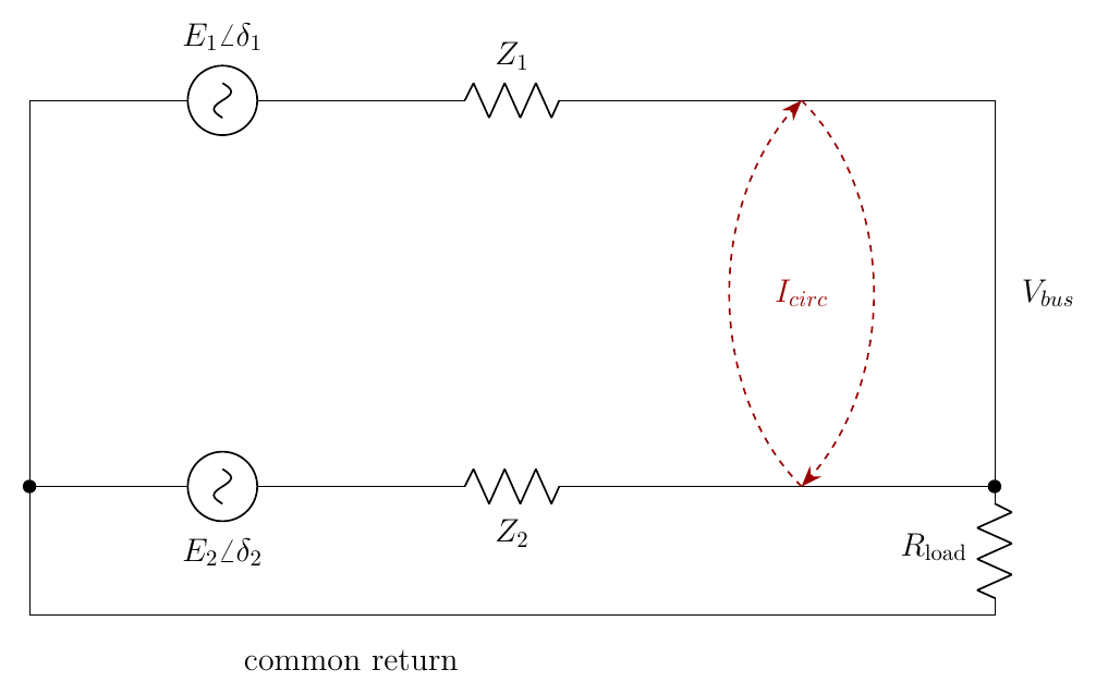
Notice that expression is the same shape as Chapter 4’s breaker-closing current: a paralleling error that persists indefinitely instead of decaying once the transient settles. An inductive \(Z\) splits it cleanly: an angle mismatch drives circulating active power (one unit effectively motors the other), and a magnitude mismatch drives circulating reactive power.
Root causes, roughly in the order they bite in practice: the steady-state Q-sharing error just derived (the largest one, and a design error rather than a fault); mismatched droop set-points or gains between units, including simple reference or measurement offsets; unequal voltage-loop dynamics during transients, even when the steady-state references agree; and, where two inverters share a common DC bus as well as a common AC bus, a low-impedance loop that circulating current can exploit almost unchecked, normally fixed with a common-mode or coupled inductor, or galvanic isolation.
Any DC component in one unit’s output voltage sees only the loop’s own winding and cable resistance (there is no reactance to limit it), and can produce a large DC circulating current between parallel single-phase units; if a transformer sits in that loop, the DC current walks its core toward saturation. A three-phase four-wire system has an analogous zero-sequence circulating current through the shared neutral, but that mechanism does not exist in single phase at all: there is no neutral wire and no sequence decomposition to speak of. The single-phase analogue is DC, not zero-sequence, and it needs an explicit DC-rejection integrator in each unit’s own controller as a standing design requirement, not an afterthought.
The X/R problem: droop’s pairing is not universal, and this is the chapter it has to be fixed in
Chapter 4 flagged this and deferred it here, because the fix belongs with the rest of this chapter’s impedance material. The exact single-line power relations for a source \(E\angle\delta\) behind \(Z = R + jX\) feeding a bus \(V\angle0\) are \[ P = \frac{V}{R^2+X^2}\Big[R(E\cos\delta - V) + XE\sin\delta\Big], \qquad Q = \frac{V}{R^2+X^2}\Big[X(E\cos\delta - V) - RE\sin\delta\Big] \]
Two small-angle limits:
- \(X \gg R\) (transmission, and the assumption behind every droop law in this book so far): \(P \approx EV\delta/X\), \(Q \approx V(E-V)/X\): the conventional pairing, \(P \leftrightarrow f\), \(Q \leftrightarrow E\).
- \(R \gg X\) (LV distribution wiring, and typically the actual case for a single-phase inverter at this book’s own scale): \(P \approx V(E-V)/R\), \(Q \approx -EV\delta/R\): the pairing inverts entirely, to \(P \leftrightarrow E\), \(Q \leftrightarrow -\delta\).
This is the single most important single-phase-relevant result in this chapter. LV feeders and domestic wiring are usually resistance-dominated: the opposite of the assumption behind the entire droop derivation in this book so far. Apply textbook P-f, Q-V droop unchanged on a genuinely resistive network, and the resulting loop is sluggish at best and positive-feedback at worst.
Two standard fixes, matching the two already met elsewhere in this book:
- Virtual inductance (Chapter 9), added purely in software so the effective output impedance is inductive at the fundamental frequency regardless of what the physical wiring is doing. In single phase, the ideal derivative form differentiates measurement noise, so the practical realisation uses one of Chapter 9’s band-limited or OSG-based routes.
- Rotated droop. Rather than fix the impedance, rotate the power pair by the line’s own impedance angle before applying conventional droop, \(P' = (XP - RQ)/|Z|\), \(Q' = (RP + XQ)/|Z|\), then droop \(\omega\) on \(P'\) and \(E\) on \(Q'\). This works for any mix of \(X\) and \(R\) and needs only the impedance’s angle, not its magnitude: a much easier thing to estimate.69 The exact normalisation above follows the conventional form used in this line of work; this book could not independently re-verify it against the original paper’s own notation, so check it against the primary source before implementing it directly.
Hierarchical control, briefly: the frame the rest of this chapter’s fixes sit inside
| Level | Job | Runs where | Communication | Timescale |
|---|---|---|---|---|
| Inner loops | Current, voltage regulation | Local | None | Sub-millisecond to a few ms |
| Primary | Droop or VSG: share P and Q, set \(\omega\) and \(E\) | Local | None | Tens to hundreds of ms |
| Secondary | Restore \(f\) and \(V\) to nominal; correct Q-sharing error | A microgrid controller | Low bandwidth | Seconds |
| Tertiary | Dispatch, economics, power flow with the wider grid | An energy management system | Full SCADA | Minutes and beyond |
Each level sits roughly an order of magnitude slower than the one below it, so the level beneath it looks like a simple algebraic gain rather than a dynamic system it has to co-design with: this is the same bandwidth-separation logic Chapter 3 introduced for the inner control cascade, one more octave up. Secondary control in its simplest form is a PI on the frequency deviation, broadcast identically to every unit: \[ \delta\omega_{sec} = k_p(\omega_0-\omega) + k_i\!\int\!(\omega_0-\omega)\,\mathrm{d}t \] added equally to every unit’s own \(\omega^*\). Because it is added equally, it shifts the whole droop family up together without disturbing the sharing ratios this chapter derived, which is exactly why the hierarchy works for frequency. The same trick for voltage genuinely does disturb the sharing ratios, which is precisely why secondary Q-sharing correction is the harder problem this chapter has already spent most of its length on.
Run two of the simulator’s droop-controlled inverters in parallel with mismatched line impedances and read the resulting reactive-power split against this chapter’s \((n_i + X_i/E)\) prediction. Then enable virtual impedance on both and watch the split converge back toward the design ratio.
Active power shares itself across parallel grid-forming inverters almost for free, because frequency is a single number the whole island agrees on with no communication link required. Reactive power does not, because voltage is a local quantity that a line drop can quietly overwhelm: the same line drop that, on the resistance-dominated wiring typical of a single-phase installation, also inverts which quantity pairs with which. Both problems, and the current-limiting problem from Chapter 8 before them, converge on the same fix: virtual impedance, deliberately overriding whatever the physical network happens to be, so the inverter’s behaviour depends on a number the designer chose rather than one the site electrician happened to install.
Where this leaves the house on its own island
Go back to the picture the Welcome opened with: the street loses power, the breaker to the grid opens, and the battery inverter in the garage is now the only thing on that little island that can set a voltage and a frequency for the house’s loads to run against. That was stated as a puzzle before any of this book had answered it. It can now be answered in full, in the order this book built it.
The voltage controller (Chapter 3) is what gives the inverter a voltage of its own to hold in the first place, by regulating the one node in the plant that actually has a state: the capacitor at the PCC. Droop (Chapter 4) is the simplest rule for what that voltage’s angle and magnitude should be, built from nothing but the inverter’s own measured power, and it turns out to already carry the inertia of a real machine without anyone asking it to. The synchronous generator (Chapter 5) is where that inertia comes from physically, and the swing equation is the one piece of mechanics a grid-forming controller borrows on purpose. The VSG (Chapter 6) builds that borrowing deliberately, trading droop’s single gain for two independent knobs, at the cost of a single-phase reactive-power path that needs real care. The governor (Chapter 7) is what turns a transient response into a permanent one. And current limiting and virtual impedance (Chapters 8 and 9) are what keep the whole arrangement alive when the island’s loads, or a fault on the way back to the grid, ask for more current than the hardware can survive, the price a voltage source pays that a current source never had to. Chapter 10 is what happens once there is more than one such inverter on the island at all.
None of that changes when the street’s power comes back and the breaker closes again: Chapter 4’s synchronising section is exactly what makes that reconnection survivable rather than a second fault in its own right. The inverter that can hold up the island on its own is, by construction, also the inverter that can rejoin the grid cleanly when the island is no longer needed.
The companion three-controller simulator, referenced throughout this book, is the place to make all of this concrete rather than read about it: build the LCL plant, choose droop or the swing equation, sweep the grid-side inductance from a stiff connection down through weak and into fully islanded, and watch the numbers in this book’s worked examples happen on your own screen. Start with the synchronisation exercise from Chapter 4: it is the cheapest way to see, in one run, why everything that came after it in this book was necessary.